cp10_Stochastics

import numpy as np
import numpy.random as npr
import matplotlib.pyplot as plt
%matplotlib inline

the rand function returns random numbers from the open interval [0,1) in the shape provided as a parameter to the function.

npr.rand(10)

 

sample_size = 500
rn1 = npr.rand(sample_size, 3)                      #Uniformly distributed random numbers in the given shape
rn2 = npr.randint(0,10,sample_size)              #Random integers for a given interval.
rn3 = npr.sample(size=sample_size)            #Uniformly distributed random numbers.
a = [0,25,50,75,100]
rn4 = npr.choice(a, size=sample_size)         #Randomly sampled values from a finite list object.

 

fig, ((ax1, ax2), (ax3, ax4)) = plt.subplots(nrows = 2, ncols=2, figsize=(7,7))

ax1.hist(rn1, bins=25, stacked = True) #stacked by columns
ax1.set_title('rand')
ax1.set_ylabel('frequency')
ax1.grid(True)

ax2.hist(rn2, bins=25)
ax2.set_title('randint')
ax2.grid(True)

ax3.hist(rn3, bins=25)
ax3.set_title('sample')
ax3.set_ylabel('frequency')
ax3.grid(True)

ax4.hist(rn4, bins=25)
ax4.set_title('choice')
ax4.grid(True)

 

#shows the results for the three continuous distributions and the discrete one (Poisson). The Poisson distribution is used, for #example, to simulate the arrival of (rare) external events, like a jump in the price of an instrument or an exogenic shock.

sample_size = 500
rn1 = npr.standard_normal(sample_size) # with mu=0, gamma=1
rn2 = npr.normal(100,20, sample_size) # with mu=100 gamma=20  (standard deviation)
rn3 = npr.chisquare(df=0.5, size=sample_size) # 0.5 degrees of freedom 
rn4 = npr.poisson(lam=1.0, size=sample_size) #lambda =1 

fig, ( (ax1, ax2), (ax3,ax4) ) = plt.subplots(nrows=2, ncols=2, figsize=(7,7) )

ax1.hist(rn1, bins=25)
ax1.set_title('standard normal')
ax1.set_ylabel('frequency')
ax1.grid(True)

ax2.hist(rn2, bins=25)
ax2.set_title('normal(100, 20)')
ax2.grid(True)

ax3.hist(rn3, bins=25)
ax3.set_title('chi square')
ax3.set_ylabel('frequency')
ax3.grid(True)

ax4.hist(rn4, bins=25)
ax4.set_title('Poisson')
ax4.grid(True)

s0 = 100 # initial value
r = 0.05 # constant short rate
sigma=0.25 # constant volatility
T=2.0 # in years
Z=10000 # number of random draws

#the level of a stock index ST1 at a future date T given a level s0 as of today is given according to Equation

ST1 = s0 * np.exp( (r-0.5 * sigma **2 )* T + sigma*np.sqrt(T) * npr.standard_normal(Z) )

plt.figure(figsize=(10,6))
plt.hist(ST1, bins=50)
plt.xlabel('index level')
plt.ylabel('frequency')

Figure suggests that the distribution of the random variable(ST1) as defined in Equation 10-1 is log-normal. We could therefore also try to use the lognormal function to directly derive the values for the random variable. In that case, we have to provide the mean and the standard deviation to the function:

s0 = 100 # initial value
r = 0.05 # constant short rate
sigma=0.25 # constant volatility
T=2.0 # in years
Z=10000 # number of random draws

#the level of a stock index ST1 at a future date T given a level s0 as of today is given according to Equation

#ST1 = s0 * np.exp( (r-0.5 * sigma **2 )* T + sigma*np.sqrt(T) * npr.standard_normal(Z) )

ST2 = s0 * npr.lognormal( (r-0.5* sigma**2)*T, #mu==mean of lognormal Distribution
                           sigma*np.sqrt(T),   #standard deviation of lognormal Distribution
                           size=Z            
                        )
plt.hist(ST2, bins=50)
plt.xlabel('index level')
plt.ylabel('frequency')
plt.grid(True)

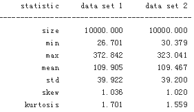
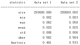
Both two figures indeed look pretty similar. But let us verify this more rigorously by comparing statistical moments of the resulting distributions.

To compare the distributional characteristics of simulation results, the scipy.stats subpackage and the helper function print_statistics(), as defined here, prove useful

import scipy.stats as scs

def print_statistics(a1, a2):
    sta1 = scs.describe(a1)
    sta2 = scs.describe(a2)
    print('%14s %14s %14s' % ('statistic', 'data set 1', 'data set 2') )
    print(45 * "-")
    print('%14s %14.3f %14.3f' % ('size', sta1[0], sta2[0]))
    print('%14s %14.3f %14.3f' % ('min', sta1[1][0], sta2[1][0]))
    print('%14s %14.3f %14.3f' % ('max', sta1[1][1], sta2[1][1]))
    print('%14s %14.3f %14.3f' % ('mean', sta1[2], sta2[2]))
    print('%14s %14.3f %14.3f' % ('std', np.sqrt(sta1[3]), np.sqrt(sta2[3])))
    print('%14s %14.3f %14.3f' % ('skew', sta1[4], sta2[4]))
    print('%14s %14.3f %14.3f' % ('kurtosis', sta1[5], sta2[5]))

print_statistics(ST1, ST2)

###########################################

help for understanding

scs.describe(ST1)

DescribeResult(nobs=10000, minmax=(28.6237705145288, 395.26905013480865), mean=110.59104586374359, variance=1677.0613219721643, skewness=1.2188387029287366, kurtosis=2.543152642124503)

###########################################

Obviously, the statistics of both simulation results are quite similar. The differences are mainly due to what is called the sampling error in simulation. Error can also be introduced when discretely simulating continuous stochastic processes — namely the discretization error, which plays no role here due to the static nature of the simulation approach.

 

Stochastic Processes

Roughly speaking, a stochastic process is a sequence of random variables. In that sense, we should expect something similar to a sequence of repeated simulations of a random variable when simulating a process. This is mainly true, apart from the fact that the draws are in general not independent but rather depend on the result(s) of the previous draw(s). In general, however, stochastic processes used in finance exhibit the Markov property, which mainly says that tomorrow’s value of the process only depends on today’s state of the process, and not any other more “historic” state or even the whole path history. The process then is also called memoryless.

Geometric Brownian motion

s0 = 100 # initial value
T=2.0 # in years
r = 0.05 # constant short rate
sigma=0.25 # constant volatility
Z=10000 # number of random draws

I =10000  #The number of paths to be simulated.
M = 50    #The number of time intervals for the discretization.
dt = T/M  #The length of the time interval in year fractions.
S = np.zeros((M+1, I) )
S[0] = s0   #first row #The initial values for the initial point in time t=0.

 

#ST1 = s0 * np.exp( (r-0.5 * sigma **2 )* T + sigma*np.sqrt(T) * npr.standard_normal(Z) )

#ST2 = s0 * npr.lognormal( (r-0.5* sigma**2)*T, #mu==mean of lognormal Distribution
#                           sigma*np.sqrt(T),   #standard deviation of lognormal Distribution
#                           size=Z            
#                        )

for t in range(1, M+1): #a stochastic process is a sequence of random variables
    S[t] = S[t-1] * np.exp((r-0.5*sigma**2)*dt + sigma*np.sqrt(dt)*npr.standard_normal(Z) )

plt.figure( figsize=(10,6) )
plt.hist(S[-1], bins=50) # the option price at maturity
plt.xlabel('index level')
plt.ylabel('frequency')

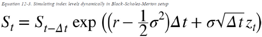
Following is a comparison of the statistics resulting from the dynamic simulation as well as from the
static simulation.

print_statistics(S[-1], ST2)

but also to value options with American/Bermudan exercise or options
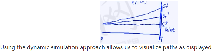
whose payoff is path-dependent. You get the full dynamic picture

#Using the dynamic simulation approach allows us to visualize paths as displayed
plt.figure(figsize=(10,6))
plt.plot(S[:, :10], lw=1.5)
plt.xlabel('time')
plt.ylabel('index level')

###########################################################################

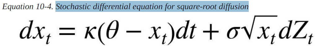
Square-root diffusion

Another important class of financial processes is mean-reverting processes, which are used to model short rates or volatility processes, for example. A popular and widely used model is the square-root diffusion, as proposed by Cox, Ingersoll, and Ross (1985). Equation 12-4 provides the respective SDE(Stochastic differential equation for square-root diffusion).

s0 = 100 # initial value
T=2.0 # in years
r = 0.05 # constant short rate
sigma=0.25 # constant volatility
Z=10000 # number of random draws

x0 = 0.05     #The initial value (e.g., for a short rate
kappa = 3.0   #The mean reversion factor
theta = 0.02  #The long-term mean value.
sigma=0.1     #The volatility factor.

The square-root diffusion has the convenient and realistic characteristic that the values of xt remain strictly positive. When discretizing it by an Euler scheme, negative values cannot be excluded. That is the reason why one works always with the positive version of the originally simulated process. In the simulation code, one therefore needs two ndarray objects instead of only one:

I = 10000   
M = 50
dt = T/M

def srd_euler():
                         #paths
    xh = np.zeros( (M+1, I) )
    xt = np.zeros_like(xh)      #xt remain strictly positive.
    xh[0] = x0  #x0 = 0.05     #The initial value (e.g., for a short rate
    xt[0] = x0
    for t in range(1,M+1):
        xh[t] = ( xh[t-1] )\
        + kappa * (theta - np.maximum(xh[t-1], 0)) * dt\
        + sigma * np.sqrt( np.maximum(xh[t-1], 0)) * np.sqrt(dt) * npr.standard_normal(I)
    print("xh: ", xh)  #actually, I saw some negative values in my first run(I took a snapshot after second run)
    xt = np.maximum(xh, 0) ## 当然 np.maximum 接受的两个参数，也可以大小一致
                           # 或者更为准确地说，第二个参数只是一个单独的值时，其实是用到了维度的 broadcast 机制；
    print("xt: ",xt)
    
    return xt

xt = srd_euler()

plt.figure(figsize=(10,6))
plt.hist(xt[-1], bins=50)
plt.xlabel('value')
plt.ylabel('frequency')

Figure then shows the first 10 simulated paths, illustrating the resulting negative, average drift (due to x0 > ) and the convergence theta to = 0.02:

plt.plot( xt[:, :10], lw=1.5)
plt.xlabel('time')            #row: time, or each column is vector
plt.ylabel('index level')     
plt.grid(True)

############################

I = 10000   
M = 50
dt = T/M

x0 = 0.05     #The initial value (e.g., for a short rate
kappa = 3.0   #The mean reversion factor
theta = 0.02  #The long-term mean value.
sigma=0.1     #The volatility factor.

def srd_exact():
    x = np.zeros((M+1, I))
    x[0] =x0
    for t in range(1, M+1):
        df = 4*theta*kappa / sigma**2    #df: degrees of freedom
        c = ( sigma**2 * (1-np.exp(-kappa * dt))) / (4*kappa)
        nc = np.exp(-kappa * dt) / c * x[t-1]  #nc: noncentrality parameter
        x[t] = c* npr.noncentral_chisquare(df, nc, size=I)
    return x

x2 = srd_exact()

plt.figure( figsize=(10,6) )
plt.hist(x2[-1], bins=50)
plt.xlabel('value')
plt.ylabel('frequency')

#presents as before the first 10 simulated paths, again displaying the negative average
#drift and the convergence to theta

plt.figure(figsize=(10,6))
plt.plot(x2[:,:10], lw=1.5)
plt.xlabel('time')
plt.ylabel('index level')

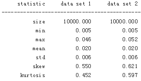
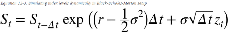
Comparing the main statistics from the different approaches reveals that the biased Euler scheme indeed performs quite well when it comes to the desired statistical properties:

print_statistics(xt[-1], x2[-1])

I = 250000
%time xt =srd_euler()

%time x2=srd_exact()

print_statistics(xt[-1], x2[-1])
xt=0.0;
x2=0.0

However, a major difference can be observed in terms of execution speed, since sampling from the noncentral chi-square distribution is more computationally demanding than from the standard normal distribution. The exact scheme takes roughly twice as much time for virtually the same results as with the Euler scheme.

Stochastic volatility

s0 = 100
r = 0.05
v0 = 0.1 #Initial (instantaneous) volatility value.
kappa = 3.0
theta = 0.25
sigma = 0.1
rho = 0.6 #Fixed correlation between the two Brownian motions.
T = 1.0

corr_mat = np.zeros((2,2))
corr_mat[0,:] = [1.0, rho]
corr_mat[1,:] = [rho, 1.0]
corr_mat

cho_mat = np.linalg.cholesky(corr_mat) #变成下三角矩阵
cho_mat

M = 50
I = 10000                     #Z  rows cols
ran_num = npr.standard_normal((2, M+1, I))

dt = T/M
v = np.zeros_like(ran_num[0])  #(M+1, I)
vh = np.zeros_like(v)   #(M+1, I)
v.shape

v[0] = v0 #0.1
vh[0] = v0

for t in range(1,M+1):           #2  M+1 i
    ran = np.dot(cho_mat, ran_num[:, t, :])
    #print(ran.shape) #(2,10000)
    vh[t] = (vh[t-1]) + kappa * (theta - np.maximum(vh[t-1], 0)) * dt \
    + sigma * np.sqrt(np.maximum(vh[t-1],0)) * np.sqrt(dt) * ran[1] #set 1 for the volatility proces 
v = np.maximum(vh,0)

S = np.zeros_like(ran_num[0])
S[0] = s0

for t in range(1, M+1):
    ran = np.dot(cho_mat, ran_num[:, t, :])                   #set 0 for the index process
    S[t] = S[t-1] * np.exp( (r-0.5*v[t])*dt + np.sqrt(v[t]) * ran[0] * np.sqrt(dt) )

fig, (ax1, ax2) = plt.subplots(1,2, figsize=(9,5))
ax1.hist(S[-1], bins=50)
ax1.set_xlabel('index level')
ax1.set_ylabel('frequency')
ax1.grid(True)

ax2.hist(v[-1], bins=50)
ax2.set_xlabel('volatility')
ax2.grid(True)

fig, (ax1, ax2) = plt.subplots(2,1, sharex=True, figsize=(7,6))
ax1.plot(S[:, :10], lw=1.5)
ax1.set_ylabel('index level')
ax1.grid(True)

ax2.plot(v[:, :10], lw=1.5)
ax2.set_xlabel('time')
ax2.set_ylabel('volatility')
ax2.grid(True)

print_statistics(S[-1], v[-1])

Finally, let us take a brief look at the statistics for the last point in time for both data sets, showing a pretty high maximum value for the index level process. In fact, this is much higher than a geometric Brownian motion with constant volatility could ever climb, ceteris paribus

Jump diffusion

Stochastic volatility and the leverage effect are stylized (empirical) facts found in a number of markets. Another important stylized fact is the existence of jumps in asset prices and, for example, volatility. In 1976, Merton published his jump diffusion model, enhancing the Black-Scholes-Merton setupthrough a model component generating jumps with log-normal distribution. The risk-neutral SDE is presented in Equation 12-8.

Poisson Distribtion (lambda, k) The Poisson distribution is popular for modelling the number of times an event occurs in an interval of time or space.λ是单位时间（或单位面积）内随机事件的平均发生率

import numpy as np
import numpy.random as npr
import matplotlib.pyplot as plt
%matplotlib inline

s0 = 100.
r = 0.05
sigma =0.2
lamb = 0.75   #The jump intensity.
mu = -0.6     #The mean jump size.
delta = 0.25  #The jump volatility.
rj = lamb * (np.exp(mu + 0.5*delta **2 )-1)  #The drift correction.

T = 1.0
M = 50
I = 10000
dt = T/M

S = np.zeros((M+1, I))
S[0] = s0
zt1 = npr.standard_normal((M+1, I))
zt2 = npr.standard_normal((M+1, I))
poi = npr.poisson(lamb*dt, (M+1, I)) #yt are Poisson distributed with intensity 

for t in range(1, M+1, 1):
    S[t] = S[t - 1] * (np.exp( (r - rj - 0.5 * sigma**2) * dt + 
                        sigma * np.sqrt(dt) * zt1[t] ) +
                        (np.exp(mu + delta * zt2[t]) -1)* poi[t]
                    )
    S[t] = np.maximum(S[t],0)

plt.figure(figsize=(10,6))
plt.hist(S[-1], bins=50)
plt.xlabel('value')
plt.ylabel('frequency')
plt.title('Dynamically simulated jump diffusion process at maturity')

Since we have assumed a highly negative mean(mu = -0.6) for the jump, it should not come as a surprise that the final values of the simulated index level are more right-skewed(mean=100, the most distribution space to right) in Figure compared to a typical log-normal distribution

the second peak (bimodal frequency distribution), which is due to the jumps

plt.figure(figsize=(10,6))
plt.plot(S[:,:10], lw=1.5)
plt.xlabel('time')
plt.ylabel('index level')

Variance Reduction

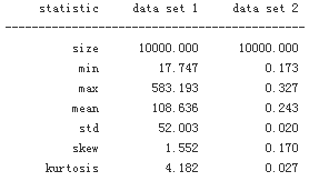
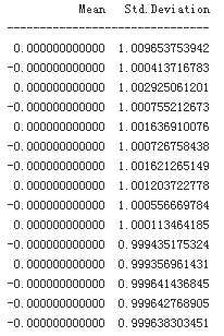
Because the Python functions used so far generate pseudo-random numbers and due to the varying sizes of the samples drawn, the resulting sets of numbers might not exhibit statistics close enough to the expected or desired ones. For example, one would expect a set of standard normally distributed random numbers to show a mean of 0 and a standard deviation of 1. Let us check what statistics different sets of random numbers exhibit. To achieve a realistic comparison, the seed value for the random number generator is fixed:

print('%15s %15s' % ('Mean', 'Std.Deviation'))
print(31 * '-')
for i in range(1,31,2):
    npr.seed(100)
    sn = npr.standard_normal(i**2 *10000)
    print('%15.12f %15.12f' % (sn.mean(), sn.std()))

i ** 2 * 10000

The results show that the statistics “somehow” get better the larger the number of draws becomes.2 But they still do not match the desired ones, even in our largest sample with more than 8,000,000 random numbers.

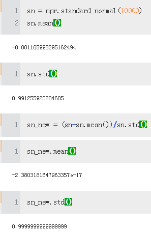
Fortunately, there are easy-to-implement, generic variance reduction techniques available to improve the matching of the first two moments of the (standard) normal distribution. The first technique is to use antithetic variates. This approach simply draws only half the desired number of random draws, and adds the same set of random numbers with the opposite sign afterward.3 For example, if the random number generator (i.e., the respective Python function) draws 0.5, then another number with value –0.5 is added to the set. By construction, the mean value of such a data set must equal zero. With NumPy this is concisely implemented by using the function np.concatenate(). The following repeats the exercise from before, this time using antithetic variates

sn = npr.standard_normal( int(10000/2 ))
sn = np.concatenate((sn, -sn)) #This concatenates the two ndarray objects
np.shape(sn)

sn.mean() #The resulting mean value is zero (within standard floating-point arithmetic errors).

print('%15s %15s' % ('Mean', 'Std.Deviation'))
print(31*'-')
for i in range(1,31,2):
    npr.seed(1000)
    sn = npr.standard_normal(i**2*10000//2)
    sn = np.concatenate((sn,-sn))
    print('%15.12f %15.12f' % (sn.mean(), sn.std()))

As immediately noticed, this approach corrects the first moment perfectly — which should not come as a surprise due to the very construction of the data set. However, this approach does not have any influence on the second moment, the standard deviation. Using another variance reduction technique, called moment matching, helps correct in one step both the first and second moments

The following function utilizes the insight with regard to variance reduction techniques and generates standard normal random numbers for process simulation using either two, one, or no variance reduction technique(s):

def gen_sn(M, I, anti_paths=True, mo_match=True):
    ''' Function to generate random numbers for simulation.
    Parameters
    ==========
    M: int
        number of time intervals for discretization
    I: int
        number of paths to be simulated
    anti_paths: boolean
        use of antithetic variates
    mo_math: boolean
        use of moment matching
    '''
    if anti_paths is True:
        sn = npr.standard_normal((M + 1, int(I / 2)))
        sn = np.concatenate((sn, -sn), axis=1)
    else:
        sn = npr.standard_normal((M + 1, I))
    if mo_match is True:
        sn = (sn - sn.mean()) / sn.std()
    return sn

 

Valuation

One of the most important applications of Monte Carlo simulation is the valuation of contingent claims(options, derivatives, hybrid instruments, etc.). Simply stated, in a risk-neutral world, the value of a contingent claim is the discounted expected payoff under the risk-neutral (martingale) measure. This is the probability measure that makes all risk factors (stocks, indices, etc.) drift at the riskless short rate, making the discounted processes martingales. According to the Fundamental Theorem of Asset Pricing, the existence of such a probability measure is equivalent to the absence of arbitrage.

A financial option embodies the right to buy (call option) or sell (put option) a specified financial instrument at a given maturity date (European option), or **over a specified period of time (American option), at a given price (strike price). Let us first consider the simpler case of European options in terms of valuation.

European Options

s0 = 100.
r = 0.05
sigma = 0.25
T = 1.0
I = 50000

def gbm_mcs_stat(K):
    ''' Valuation of European call option in Black-Scholes-Merton
    by Monte Carlo simulation (of index level at maturity)
    Parameters
    ==========
    K: float
        (positive) strike price of the option
    Returns
    =======
    C0: float
        estimated present value of European call option
    '''
    sn = gen_sn(1, I)   #gen_sn(M, I, anti_paths=True, mo_match=True): return sn
    # simulate index level at maturity
    ST = s0 * np.exp( (r-0.5*sigma**2)*T + sigma*np.sqrt(T)*sn[1] )
    
    # Calculate payoff at maturity
    hT = np.maximum(ST - K, 0)
    
    # Calculate MCS estimator
    C0 = np.exp(-r*T) * np.mean(hT) #############
    
    return C0

gbm_mcs_stat(K=105.) #The Monte Carlo estimator value for the European call option.

##################################################

Next, consider the dynamic simulation approach(better) and allow for European put options in addition to the call option. The function gbm_mcs_dyna() implements the algorithm. The code also compares option price estimates for a call and a put stroke at the same level:

 

M = 50 #The number of time intervals for the discretization.

def gbm_mcs_dyna(K, option = 'call'):
    ''' Valuation of European options in Black-Scholes-Merton
    by Monte Carlo simulation (of index level paths)
    Parameters
    ==========
    K: float
        (positive) strike price of the option
    option : string
        type of the option to be valued ('call', 'put')
    Returns
    =======
    C0: float
        estimated present value of European call option
    '''
    dt = T/M
    # simulation of index level paths
    S = np.zeros((M+1, I))
    S[0] = s0 #100 
    sn = gen_sn(M,I)
    for t in range(1, M+1, 1):
        S[t] = S[t-1] * np.exp( (r-0.5*sigma**2)*dt + sigma*np.sqrt(dt)*sn[t] )
        
    # case-based calculation of payoff
    if option == 'call':
        hT = np.maximum(S[-1]-K, 0)
    else:
        hT = np.maximum(K-S[-1],0)
    
    # Calculation of MCS estimator
    c0 = np.exp(-r * T) * np.mean(hT)
    return c0

 

gbm_mcs_dyna(K=110., option = 'call') #The Monte Carlo estimator value for the European call option.

gbm_mcs_dyna(K=110., option='put') #The Monte Carlo estimator value for the European put option.

The question is how well these simulation-based valuation approaches perform relative to the benchmark value from the Black-Scholes-Merton valuation formula. To find out, the following code generates respective option values/estimates for a range of strike prices, using the analytical option pricing formula for European calls found in the module bsm_functions.py

from bsm_functions import bsm_call_value

def bsm_call_value(S0, K, T, r, sigma):
    ''' Valuation of European call option in BSM model.
    Analytical formula.

    Parameters
    ==========
    S0: float
        initial stock/index level
    K: float
        strike price
    T: float
        maturity date (in year fractions)
    r: float
        constant risk-free short rate
    sigma: float
        volatility factor in diffusion term

    Returns
    =======
    value: float
        present value of the European call option
    '''
    from math import log, sqrt, exp
    from scipy import stats

    S0 = float(S0)
    d1 = (log(S0 / K) + (r + 0.5 * sigma ** 2) * T) / (sigma * sqrt(T))
    d2 = (log(S0 / K) + (r - 0.5 * sigma ** 2) * T) / (sigma * sqrt(T))
    # stats.norm.cdf --> cumulative distribution function
    #                    for normal distribution
    value = (S0 * stats.norm.cdf(d1, 0.0, 1.0) -
             K * exp(-r * T) * stats.norm.cdf(d2, 0.0, 1.0))
    return value

 

stat_res = []
dyna_res = []
anal_res = []
k_list = np.arange(80.,120.1, 5.)
np.random.seed(200000)
for K in k_list:
    stat_res.append(gbm_mcs_stat(K))
    dyna_res.append(gbm_mcs_dyna(K))
    anal_res.append(bsm_call_value(s0, K, T, r, sigma))
stat_res = np.array(stat_res)
dyna_res = np.array(dyna_res)
anal_res = np.array(anal_res)

 

fig, (ax1, ax2) = plt.subplots(2,1, sharex = True, figsize=(8,6))

ax1.plot(k_list, anal_res, 'b', label = 'analytical')
ax1.plot(k_list, stat_res, 'ro', label = 'static')
ax1.set_ylabel('European call option value')
ax1.grid(True)
ax1.legend(loc=0)
ax1.set_ylim(ymin=0)

wi = 1.0

ax2.bar(k_list - wi /2, (anal_res - stat_res)/anal_res*100, wi)
ax2.set_xlabel('strike')
ax2.set_ylabel('difference in %')
ax2.set_xlim(left=75, right=125)
ax2.grid(True)

plt.title("Comparison of static and dynamic Monte Carlo estimator values")

Again, all valuation differences are smaller than 1%, absolutely with both positive and negative deviations. As a general rule, the quality of the Monte Carlo estimator can be controlled for by adjusting the number of time intervals M used and/or the number of paths I simulated:

k_list - wi /2

fig, (ax1, ax2) = plt.subplots(2,1, sharex=True, figsize=(8,6))

ax1.plot(k_list, anal_res, 'b', label='analytical')
ax1.plot(k_list, dyna_res, 'ro', label='dynamic')
ax1.set_ylabel('European call option value')
ax1.grid(True)
ax1.legend(loc=0)
ax1.set_ylim(ymin=0)

wi=1.0

ax2.bar(k_list-wi/2, (anal_res - dyna_res)/anal_res*100, wi)
ax2.set_xlabel('strike')
ax2.set_ylabel('difference in %')
ax2.set_xlim(left=75, right=125)
ax2.grid(True)

American Options

################################################

Real World Example of an American Option

An investor purchased an American style call option for Apple Inc. (AAPL) in March with an expiration date at the end of December in the same year. The premium is $5 per option contract—one contract is 100 shares ($5 x 100 = $500)—and the strike price on the option is $100. Following the purchase, the stock price rose to $150 per share.

The investor exercises the call option on Apple before expiration buying 100 shares of Apple for $100 per share. In other words, the investor would be long 100 shares of Apple at the $100 strike price. The investor immediately sells the shares for the current market price of $150 and pockets the $50 per share profit. The investor earned $5,000 in total minus the premium of $500 for buying the option and any broker commissions.

Let's say an investor believes shares of Facebook Inc. (FB) will decline in the upcoming months. The investor purchases an American style July put option in January, which expires in September of the same year. The option premium is $3 per contract (100 x $3 = $300) and the strike price is $150.

Facebook's stock price falls to $90 per share, and the investor exercises the put option and is short 100 shares of Facebook at the $150 strike price. The transaction effectively has the investor buying 100 shares of Facebook at the current $90 price and immediately selling those shares at the $150 strike price. However, in practice, the net difference is settled, and the investor earns a $60 profit on the option contract, which equates to $6,000 minus the premium of $300 and any broker commissions

################################################

s0 = 100.
r = 0.05
sigma = 0.25
T = 1.0
I = 50000
M = 50 #The number of time intervals for the discretization.

 

def gbm_mcs_amer(K, option='call'):
    ''' Valuation of American option in Black-Scholes-Merton
    by Monte Carlo simulation by LSM algorithm
    Parameters
    ==========
    K : float
        (positive) strike price of the option
    option : string
        type of the option to be valued ('call', 'put')
    Returns
    =======
    C0 : float
        estimated present value of European call option
    '''
    dt = T/M
    df = np.exp(-r * dt)
    # simulation of index levels
    S = np.zeros((M+1, I))
    S[0] = s0
    sn = gen_sn(M,I)
    for t in range(1,M+1): # market price at time t
        S[t] = S[t-1] * np.exp( (r-0.5*sigma**2)*dt + sigma*np.sqrt(dt)*sn[t] )
    # case based calculation of payoff (profit after excuting)                                     ###### ht(s)
    if option == 'call':
        h = np.maximum(S-K, 0)  #market price > strike price
    else:
        h = np.maximum(K-S, 0)  #strike price > market price
    # LSM algorim
    V = np.copy(h)  #Non-execution value 
    for t in range(M-1, 0, -1):
                              # V[t+1]*df : next period American option price[see equation] 
        reg = np.polyfit(S[t], V[t+1]*df, 7) #7: arbitrary value 
        C = np.polyval(reg, S[t]) #continuation value of the option given an index level of St = s. ###### Ct(s)
        #the value of an American (Bermudan) option at any given date t is given as Vt(s) = max(ht(s),Ct(s)),
#if next period American option price > the profit at time t(stike price), we will not to execute ### h[t]:excise
        V[t] = np.where( C>h[t], V[t+1]*df, h[t] )
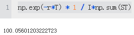
    # MCS estimator
    C0 = df * np.mean(V[1]) #C0 = df * 1 / I * np.sum(V[1]) # V[1]: the last second value
    return C0

 

gbm_mcs_amer(110, option='call') #strike price=110

gbm_mcs_amer(110, option='put')

The European value of an option represents a lower bound to the (dynamic)American option’s value. The difference is generally called the early exercise premium. What follows compares European and American option values for the same range of strikes as before to estimate the early exercise premium, this time with puts:

euro_res = []
amer_res = []

k_list = np.arange(80., 120.1, 5.)

for K in k_list:
    euro_res.append(gbm_mcs_dyna(K,'put'))
    amer_res.append(gbm_mcs_amer(K,'put'))
    
euro_res = np.array(euro_res)
amer_res = np.array(amer_res)

fig, (ax1, ax2) = plt.subplots(2, 1, sharex=True, figsize=(10, 6))
ax1.plot(k_list, euro_res, 'b', label='European put')
ax1.plot(k_list, amer_res, 'ro', label='American put')
ax1.set_ylabel('call option value')
ax1.legend(loc=0)
wi = 1.0
ax2.bar(k_list - wi / 2, (amer_res - euro_res) / euro_res * 100, wi)
ax2.set_xlabel('strike')
ax2.set_ylabel('early exercise premium in %')
ax2.set_xlim(left=75, right=125);

Risk Measures

Value-at-Risk

Value-at-risk (VaR) is one of the most widely used risk measures, and a much debated one. Loved by practitioners for its intuitive appeal, it is widely discussed and criticized by many — mainly on theoretical grounds, with regard to its limited ability to capture what is called tail risk (more on this shortly). In words, VaR is a number denoted in currency units (e.g., USD, EUR, JPY) indicating a loss (of a portfolio, a single position, etc.) that is not exceeded with some confidence level (probability) over a given period of time.

Consider a stock position, worth 1 million USD today, that has a VaR of 50,000 USD at a confidence level of 99% over a time period of 30 days (one month). This VaR figure says that with a probability of 99% (i.e., in 99 out of 100 cases), the loss to be expected over a period of 30 days will not exceed 50,000 USD. However, it does not say anything about the size of the loss once a loss beyond 50,000 USD occurs — i.e., if the maximum loss is 100,000 or 500,000 USD what the probability of such a specific “higher than VaR loss” is. All it says is that there is a 1% probability that a loss of a minimum of 50,000 USD or higher will occur.

Assume again that we are in a Black-Scholes-Merton setup and consider the following parameterization and simulation of index levels at a future date T = 30/365 (i.e., we assume a period of 30 days):

import numpy as np
import numpy.random as npr
import matplotlib.pyplot as plt
%matplotlib inline
import scipy.stats as scs

s0 = 100
r = 0.05
sigma = 0.25
T = 30/365.
I = 10000

To estimate VaR figures, we need the simulated absolute profits and losses relative to the value of the position today in a sorted manner, i.e., from the severest loss to the largest profit

#Simulates end-of-period values for the geometric Brownian motion.
ST = s0 * np.exp( (r-0.5*sigma**2)*T + sigma*np.sqrt(T)*npr.standard_normal(I) )

#Calculates the absolute profits and losses per simulation run and sorts the values.
R_gbm = np.sort(ST - s0)

plt.figure( figsize=(10,6) )
plt.hist(R_gbm, bins = 50)
plt.xlabel('absolute return')
plt.ylabel('frequency')
plt.title("Absolute profits and losses from simulation (geometric Brownian motion)")
plt.show()

Having the ndarray object with the sorted results, the function scoreatpercentile already does the trick. All we have to do is to define the percentiles (in percent values) in which we are interested. In the list object percs, 0.1 translates into a confidence level of 100% – 0.1% = 99.9%. The 30-day VaR given a confidence level of 99.9% in this case is 20.2 currency units, while it is 8.9 at the 90% confidence level

percs = [0.01, 0.1, 1., 2.5, 5.0, 10.0]
var = scs.scoreatpercentile(R_gbm, percs)
print("%16s %16s" % ('Confidence Level', 'Value-at-Risk'))
print(33*"-")

for pair in zip(percs, var):
    print("%16.2f %16.3f" % (100-pair[0], -pair[1]))

s0 = 100
r = 0.05
sigma = 0.25
T = 30/365.  #T default 1 year
I = 10000

M = 50
mu = -0.6     #The mean jump size.
delta = 0.25  #The jump volatility.

dt = 30./365/M
lamb = 0.75   #The jump intensity.
rj = lamb * (np.exp(mu + 0.5*delta **2 )-1)  #The drift correction.
S = np.zeros((M+1, I))
S[0] = s0
sn1 = npr.standard_normal((M+1, I))
sn2 = npr.standard_normal((M+1, I))
poi = npr.poisson(lamb*dt, (M+1, I))
for t in range(1,M+1,1):
    S[t] = S[t-1] * (np.exp( (r-rj-0.5*sigma**2)*dt
                             + sigma * np.sqrt(dt)*sn1[t]
                           )
                     + (np.exp(mu + delta*sn2[t])-1)
                     * poi[t]
                    )
    S[t] = np.maximum(S[t],0)

R_jd = np.sort(S[-1]-s0)

 

plt.hist(R_jd, bins=50)
plt.xlabel('absolute return')
plt.ylabel('frequency')
plt.grid(True)
plt.title("Absolute returns of jump diffusion (30d)")

For this process and parameterization, the VaR over 30 days at the 90% level is almost identical(8.982 VS 8.942), while it is more than three times as high at the 99.9% level as with the geometric Brownian motion (71 vs. 20.2 currency units)

percs = [0.01, 0.1, 1., 2.5, 5.0, 10.0]
var = scs.scoreatpercentile(R_jd, percs)
print("%16s %16s" % ('Confidence Level', 'Value-at-Risk'))
print(33*"-")
for pair in zip(percs, var):
    print("%16.2f %16.3f" % (100-pair[0], -pair[1]))

percs = list(np.arange(0.0, 10.1, 0.1))
gbm_var = scs.scoreatpercentile(R_gbm, percs)
jd_var = scs.scoreatpercentile(R_jd, percs)

This illustrates the problem of capturing the tail risk so often encountered in financial markets by the standard VaR measure

plt.plot(percs, gbm_var, 'b', lw=1.5, label='GBM')
plt.plot(percs, jd_var, 'r', lw=1.5, label='JD')

plt.legend(loc=4)
plt.xlabel('100-confidence level [%]')
plt.ylabel('value-at-risk')
plt.grid(True)
plt.ylim(ymax=0.0)
plt.title('Value-at-risk for geometric Brownian motion and jump diffusion')

Credit Valuation Adjustments

Other important risk measures are the credit value-at-risk (CVaR) and the credit valuation adjustment (CVA), which is derived from the CVaR. Roughly speaking, CVaR is a measure for the risk resulting from the possibility that a counterparty might not be able to honor its obligations — for example, if the counterparty goes bankrupt. In such a case there are two main assumptions to be made: theprobability of default and the (average) loss level.

s0 = 100.
r = 0.05
sigma = 0.2
T = 1
I = 100000
ST = s0 * np.exp((r-0.5*sigma**2)*T
                + sigma * np.sqrt(T) * npr.standard_normal(I)
                )

In the simplest case, one considers a fixed (average) loss level L and a fixed probability p for default (per year) of a counterparty:

L = 0.5  #Defines the loss level.
p = 0.01 #Defines the probability of default.

Using the Poisson distribution, default scenarios are generated as follows, taking into account that a default can only occur once

D = npr.poisson(p*T, I)  #Simulates default events.
D = np.where(D>1, 1, D)  #Limits defaults to one such event.

Without default, the risk-neutral value of the future index level should be equal to the current value of the asset today (up to differences resulting from numerical errors):

The CVaR under our assumptions is calculated as follows:

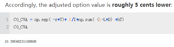
the present value of the asset, adjusted for the credit risk, is given as follows:

This should be (roughly) the same as subtracting the CVaR value from the current asset value:

In this particular simulation example, we observe roughly 1,000 losses due to credit risk, which is to be expected given the assumed default probability of 1%(p = 0.01 #Defines the probability of default.) and 100,000 simulated paths:

shows the complete frequency distribution of the losses due to a default. Of course, in the large majority of cases (i.e., in about 99,000 of the 100,000 cases(I=100000)) there is no loss to observe:

plt.hist(L*D*ST, bins=50)
plt.xlabel('loss')
plt.ylabel('frequency')
plt.grid(True)
plt.ylim(ymax=175)
plt.title('Losses due to risk-neutrally expected default (stock)')

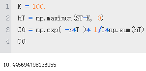
Consider now the case of a European call option. Its value is about 10.4 currency units at a strike of 100:

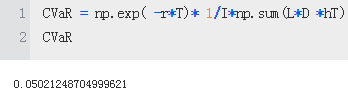
The CVaR is about 5 cents given the same assumptions with regard to probability of default and loss level:

Compared to the case of a regular asset, the option case has somewhat different characteristics. We only see a little more than 500 losses due to a default, although we again have about 1,000 defaults. This results from the fact that the payoff of the option at maturity has a high probability of being zero

shows that the CVaR for the option has a completely different frequency distribution compared to the regular asset case