【笔记】扩散模型（二）：DDIM 理论推导与代码实现

论文链接：Denoising Diffusion Implicit Models

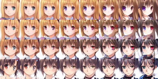
在正式开始之前先贴一个生成结果示例：

在上一篇文章中我们进行了 DDPM 的理论推导，并且自己编写代码实现了 DDPM 的训练和采样过程。虽然取得了还不错的效果，但 DDPM 有一个非常明显的问题：采样过程很慢。因为 DDPM 的反向过程利用了马尔可夫假设，所以每次都必须在相邻的时间步之间进行去噪，而不能跳过中间步骤。原始论文使用了 1000 个时间步，所以我们在采样时也需要循环 1000 次去噪过程，这个过程是非常慢的。

为了加速 DDPM 的采样过程，DDIM 在不利用马尔可夫假设的情况下推导出了 diffusion 的反向过程，最终可以实现仅采样 20～100 步的情况下达到和 DDPM 采样 1000 步相近的生成效果，也就是提速 10～50 倍。这篇文章将对 DDIM 的理论进行讲解，并实现 DDIM 采样的代码。

DDPM 的反向过程

首先我们回顾一下 DDPM 反向过程的推导，为了推导出 $q({\mathbf{x}}_{t-1}|{\mathbf{x}}_t)$ 这个条件概率分布，DDPM 利用贝叶斯公式将其变成了先验分布的组合，并且通过向条件中加入 ${\mathbf{x}}_0$ 将所有的分布转换为已知分布：
$$q({\mathbf{x}}_{t-1}|{\mathbf{x}}_t,{\mathbf{x}}_0)=\frac{q({\mathbf{x}}_t|{\mathbf{x}}_{t-1},{\mathbf{x}}_0)q({\mathbf{x}}_{t-1}|{\mathbf{x}}_0)}{q({\mathbf{x}}_t|{\mathbf{x}}_0)}$$
在上边这个等式的右侧，$q({\mathbf{x}}_{t-1}|{\mathbf{x}}_0)$ 和 $q({\mathbf{x}}_t|{\mathbf{x}}_0)$ 都是已知的，需要求解的只有 $q({\mathbf{x}}_t|{\mathbf{x}}_{t-1},{\mathbf{x}}_0)$。在这里 DDPM 引入马尔可夫假设，认为 ${\mathbf{x}}_t$ 只与 ${\mathbf{x}}_{t-1}$ 有关，将其转化成了 $q({\mathbf{x}}_t|{\mathbf{x}}_{t-1})$。最后经过推导，得出条件概率分布：
$$q({\mathbf{x}}_{t-1}|{\mathbf{x}}_t)=\mathcal{N}({\mathbf{x}}_{t-1};{\mu }_{\theta }({\mathbf{x}}_t,t),{\sigma }_t^2\mathbf{I})$$
我们可以看到之所以 DDPM 很慢，就是因为在推导 $q({\mathbf{x}}_t|{\mathbf{x}}_{t-1},{\mathbf{x}}_0)$ 的时候引入了马尔可夫假设，使得去噪只能在相邻时间步之间进行。如果我们可以在不依赖马尔可夫假设的情况下推导出 $q({\mathbf{x}}_{t-1}|{\mathbf{x}}_t,{\mathbf{x}}_0)$，就可以将上面式子里的 $t-1$ 替换为任意的中间时间步 $\tau$，从而实现采样加速。总结来说，DDIM 主要有两个出发点：

1. 保持前向过程的分布 $q({\mathbf{x}}_t|{\mathbf{x}}_{t-1})=\mathcal{N}\left({\mathbf{x}}_t;\sqrt{{\bar{\alpha }}_t}{\mathbf{x}}_0,(1-{\bar{\alpha }}_t)\mathbf{I}\right)$ 不变；
2. 构建一个不依赖于马尔可夫假设的 $q({\mathbf{x}}_{\tau }|{\mathbf{x}}_t,{\mathbf{x}}_0)$ 分布。

$q({\mathbf{x}}_{\tau }|{\mathbf{x}}_t,{\mathbf{x}}_0)$ 的推导

开始推导之前简单说明一下，这个 $q({\mathbf{x}}_{\tau }|{\mathbf{x}}_t,{\mathbf{x}}_0)$ 实际上就是上一章中提到的 $q({\mathbf{x}}_{t-1}|{\mathbf{x}}_t,{\mathbf{x}}_0)$，只不过是因为我们的推导不再依赖马尔可夫假设，所以 $t-1$ 可以替换为任意的 $\tau \in (0,t)$。为了避免混淆，我们在这里使用一个通用的符号 $\tau \in (0,t)$ 表示中间的时间步。

另一点需要说明的是，在 DDIM 的论文中，$\alpha$ 表示的含义和 DDPM 论文中的 $\bar{\alpha }$ 相同。为了保证前后一致，我们在这里依然使用 DDPM 的符号约定，令 ${\alpha }_t=1-{\beta }_t$，${\bar{\alpha }}_t={\prod }_{i=1}^t{\alpha }_i$。

我们在 DDPM 里已经推导出了 $q({\mathbf{x}}_{t-1}|{\mathbf{x}}_t,{\mathbf{x}}_0)$ 是一个高斯分布，均值和方差为：
$$\begin{array}{rl}\mu & =\frac{\sqrt{{\alpha }_t}(1-{\bar{\alpha }}_{t-1})}{1-{\bar{\alpha }}_t}{\mathbf{x}}_t+\frac{\sqrt{{\bar{\alpha }}_{t-1}}{\beta }_t}{1-{\bar{\alpha }}_t}{\mathbf{x}}_0\\ \sigma & ={\left(\frac{{\alpha }_t}{{\beta }_t}+\frac{1}{1-{\bar{\alpha }}_{t-1}}\right)}^{-1/2}\end{array}$$
可以看到均值是 ${\mathbf{x}}_0$ 与 ${\mathbf{x}}_t$ 的线性组合，方差是时间步的函数。DDIM 基于这样的规律，使用待定系数法：
$$q({\mathbf{x}}_{\tau }|{\mathbf{x}}_t,{\mathbf{x}}_0)=\mathcal{N}({\mathbf{x}}_{\tau };\lambda {\mathbf{x}}_0+k{\mathbf{x}}_t,{\sigma }_t^2\mathbf{I})$$
也就是 ${\mathbf{x}}_{\tau }=\lambda {\mathbf{x}}_0+k{\mathbf{x}}_t+{\sigma }_t{ϵ}_{\tau }$。又因为前向过程满足 ${\mathbf{x}}_t=\sqrt{{\bar{\alpha }}_t}{\mathbf{x}}_0+\sqrt{1-{\bar{\alpha }}_t}{ϵ}_t$，代入可以得到：
$$\begin{array}{rl}{\mathbf{x}}_{\tau }& =\lambda {\mathbf{x}}_0+k{\mathbf{x}}_t+{\sigma }_t{ϵ}_{\tau }\\ & =\lambda {\mathbf{x}}_0+k(\sqrt{{\bar{\alpha }}_t}{\mathbf{x}}_0+\sqrt{1-{\bar{\alpha }}_t}{ϵ}_t)+{\sigma }_t{ϵ}_{\tau }\\ & =(\lambda +k\sqrt{{\bar{\alpha }}_t}){\mathbf{x}}_0+(k\sqrt{1-{\bar{\alpha }}_t}{ϵ}_t+{\sigma }_t{ϵ}_{\tau })\\ & =(\lambda +k\sqrt{{\bar{\alpha }}_t}){\mathbf{x}}_0+\sqrt{k^2(1-{\bar{\alpha }}_t)+{\sigma }_t^2}ϵ\end{array}$$
在上面的推导过程中，由于 ${ϵ}_t$ 和 ${ϵ}_{\tau }$ 都满足标准正态分布，因此两项可以合并。又因为根据前向过程，有 ${\mathbf{x}}_{\tau }=\sqrt{{\bar{\alpha }}_{\tau }}{\mathbf{x}}_0+\sqrt{1-{\bar{\alpha }}_{\tau }}{ϵ}_{\tau }$，将两个式子的系数对比，可以得到方程组：
$$\{\begin{array}{l}\begin{array}{rl}\lambda +k\sqrt{{\bar{\alpha }}_t}& =\sqrt{{\bar{\alpha }}_{\tau }}\\ \sqrt{k^2(1-{\bar{\alpha }}_t)+{\sigma }_t^2}& =\sqrt{1-{\bar{\alpha }}_{\tau }}\end{array}\end{array}$$
解方程组得到 $\lambda$ 和 $k$：
$$\{\begin{array}{l}\begin{array}{rl}\lambda & =\sqrt{{\bar{\alpha }}_{\tau }}-\sqrt{\frac{(1-{\bar{\alpha }}_{\tau }-{\sigma }_t^2){\bar{\alpha }}_t}{1-{\bar{\alpha }}_t}}\\ k& =\sqrt{\frac{1-{\bar{\alpha }}_{\tau }-{\sigma }_t^2}{1-{\bar{\alpha }}_t}}\end{array}\end{array}$$
在上边的结果中，我们得到了 $q({\mathbf{x}}_{\tau }|{\mathbf{x}}_t,{\mathbf{x}}_0)$ 均值中的两个参数，而方差 ${\sigma }_t^2$ 并没有唯一定值，因此这个结果对应于一组解，通过规定不同的方差，可以得到不同的采样过程。我们把 ${\mathbf{x}}_0$ 用 ${\mathbf{x}}_t$ 替换，可以得到均值的表达式：
$$\begin{array}{rl}\mu & =\lambda {\mathbf{x}}_0+k{\mathbf{x}}_t\\ & =\left(\sqrt{{\bar{\alpha }}_{\tau }}-\sqrt{\frac{(1-{\bar{\alpha }}_{\tau }-{\sigma }_t^2){\bar{\alpha }}_t}{1-{\bar{\alpha }}_t}}\right){\mathbf{x}}_0+\sqrt{\frac{1-{\bar{\alpha }}_{\tau }-{\sigma }_t^2}{1-{\bar{\alpha }}_t}}{\mathbf{x}}_t\\ & =\left(\sqrt{{\bar{\alpha }}_{\tau }}-\sqrt{\frac{(1-{\bar{\alpha }}_{\tau }-{\sigma }_t^2){\bar{\alpha }}_t}{1-{\bar{\alpha }}_t}}\right)\left(\frac{{\mathbf{x}}_t-\sqrt{1-{\bar{\alpha }}_t}{ϵ}_{\theta }({\mathbf{x}}_t,t)}{\sqrt{{\bar{\alpha }}_t}}\right)+\sqrt{\frac{1-{\bar{\alpha }}_{\tau }-{\sigma }_t^2}{1-{\bar{\alpha }}_t}}{\mathbf{x}}_t\\ & =\sqrt{{\bar{\alpha }}_{\tau }}\frac{{\mathbf{x}}_t-\sqrt{1-{\bar{\alpha }}_t}{ϵ}_{\theta }({\mathbf{x}}_t,t)}{\sqrt{{\bar{\alpha }}_t}}+\sqrt{1-{\bar{\alpha }}_{\tau }-{\sigma }_t^2}{ϵ}_{\theta }({\mathbf{x}}_t,t)\end{array}$$
因此我们可以得到最终的 ${\mathbf{x}}_{\tau }$ 的表达式：
$$\begin{array}{rl}{\mathbf{x}}_{\tau }& =\mu +{\sigma }_tϵ\\ & =\sqrt{{\bar{\alpha }}_{\tau }}\underset{预测的{\mathbf{x}}_0}{\underbrace{\frac{{\mathbf{x}}_t-\sqrt{1-{\bar{\alpha }}_t}{ϵ}_{\theta }({\mathbf{x}}_t,t)}{\sqrt{{\bar{\alpha }}_t}}}}+\underset{指向{\mathbf{x}}_t的方向}{\underbrace{\sqrt{1-{\bar{\alpha }}_{\tau }-{\sigma }_t^2}{ϵ}_{\theta }({\mathbf{x}}_t,t)}}+\underset{随机的噪声}{\underbrace{{\sigma }_tϵ}}\end{array}$$

方差的取值

正如我们前文中所说，我们得到的实际上是 ${\mathbf{x}}_{\tau }$ 的一组解，其中的 ${\sigma }_t$ 并没有固定的取值。在论文中，作者参照 DDPM 的方差的形式给出了一个 ${\sigma }_t$ 的形式：
$${\sigma }_t=\eta \sqrt{\frac{1-{\bar{\alpha }}_{\tau }}{1-{\bar{\alpha }}_t}}\sqrt{1-{\alpha }_t}$$

1. 当 $\eta =1$，生成过程与 DDPM 一致。这个感觉还是可以理解的，因为在待定系数法求解时，本身就是假定均值的形式和 DDPM 相同，如果再假定方差和 DDPM 相同，那么最后的整体形式也会变成 DDPM。
2. 当 $\eta =0$，此时生成过程不再添加随机噪声项，唯一带有随机性的因素就是采样初始的 ${\mathbf{x}}_T\sim \mathcal{N}(0,1)$，因此采样的过程是确定的，每个 ${\mathbf{x}}_T$ 对应唯一的 ${\mathbf{x}}_0$，这个模型就是 DDIM。

采样加速

我们知道 DDIM 的反向过程并不依赖于马尔可夫假设，因此去噪的过程并不需要在相邻的时间步之间进行，也就是跳过一些中间的步骤。形式化地来说，DDPM 的采样时间步应当是 $[T,T-1,...,2,1]$，而 DDIM 可以直接从其中抽取一个子序列 $[{\tau }_S,{\tau }_{S-1},...,{\tau }_2,{\tau }_1]$ 进行采样。

在 DDIM 论文的附录中，给出了两种子序列的选取方式：

• 线性选取：令 ${\tau }_i=\lfloor ci\rfloor$
• 二次方选取：令 ${\tau }_i=\lfloor c{i}^2\rfloor$

其中 $c$ 是一个常量，制定这个常量的规则是让 ${\tau }_{-1}$ 也就是最后一个采样时间步尽可能与 $T$ 接近。在原文的实验中，CIFAR10 使用的是二次方选取，其他数据集都使用的是线性选取方式。

DDIM 区别于 DDPM 的两个特性

1. 采样一致性：我们知道 DDIM 的采样过程是确定的，生成结果只受 ${\mathbf{x}}_T$ 影响。作者经过实验发现对于同一个 ${\mathbf{x}}_T$，使用不同的采样过程，最终生成的 ${\mathbf{x}}_0$ 比较相近，因此 ${\mathbf{x}}_T$ 在一定程度上可以看作 ${\mathbf{x}}_0$ 的一种嵌入。

   因为这个性质的存在，在生成图像时也有一个 trick。也就是一开始先选取一个较小的时间步数量生成比较粗糙的图像，如果大致样子符合预期，再使用大时间步数量进行精细生成。

2. 语义插值效应：根据上一条性质，${\mathbf{x}}_T$ 可以看作 ${\mathbf{x}}_0$ 的嵌入，那么它可能也具有其他隐概率模型所具有的语义差值效应。作者首先选取两个隐变量 ${\mathbf{x}}_T^{(0)}$ 和 ${\mathbf{x}}_T^{(1)}$，对其分别采样得到结果，然后使用球面线性插值得到一系列中间隐变量，这个插值定义为：
   $${\mathbf{x}}_T^{(\alpha )}=\frac{\sin (1-\alpha )\theta }{\sin \theta }{\mathbf{x}}_T^{(0)}+\frac{\sin \alpha \theta }{\sin \theta }{\mathbf{x}}_T^{(1)}$$
   其中 $\theta =\arccos \left(\frac{({\mathbf{x}}_T^{(0)}{)}^T{\mathbf{x}}_T^{(1)}}{||{\mathbf{x}}_T^{(0)}||||{\mathbf{x}}_T^{(1)}||}\right)$。最终也在 DDIM 上观察到了语义插值效应，我们下面也将复现这一实验。

DDIM 的代码实现

从上面的推导过程可以发现，DDIM 假设的前向过程和 DDPM 相同，只有采样过程不同。因此想把 DDPM 改成 DDIM 并不需要重新训练，只要修改采样过程就可以了。在上一篇文章中我们已经训练好了一个 DDPM 模型，这里我们继续用这个训练好的模型来构造 DDIM 的采样过程。

如果你没有看上一篇文章，也可以直接在这个链接直接下载训练好的权重。

我们把训练好的 DDPM 模型的权重加载进来用作噪声预测网络：

from diffusers import UNet2DModel

model = UNet2DModel.from_pretrained('ddpm-anime-faces-64').cuda()

核心代码

首先我们依然是定义一系列常量，$\alpha$、$\beta$ 等都和 DDPM 相同，只有采样的时间步不同。我们在这里直接线性选取 20 个时间步，最大的为 999，最小的为 0：

import torch

class DDIM:
    def __init__(
        self,
        num_train_timesteps:int = 1000,
        beta_start: float = 0.0001,
        beta_end: float = 0.02,
        sample_steps: int = 20,
    ):
        self.num_train_timesteps = num_train_timesteps
        self.betas = torch.linspace(beta_start, beta_end, num_train_timesteps, dtype=torch.float32)
        self.alphas = 1.0 - self.betas
        self.alphas_cumprod = torch.cumprod(self.alphas, dim=0)
        self.timesteps = torch.linspace(num_train_timesteps - 1, 0, sample_steps).long()

然后是实现采样过程，和 DDPM 一样，我们把需要的公式复制到这里，然后对照着实现：
$$\begin{array}{rl}{\mathbf{x}}_{\tau }& =\sqrt{{\bar{\alpha }}_{\tau }}\frac{{\mathbf{x}}_t-\sqrt{1-{\bar{\alpha }}_t}{ϵ}_{\theta }({\mathbf{x}}_t,t)}{\sqrt{{\bar{\alpha }}_t}}+\sqrt{1-{\bar{\alpha }}_{\tau }-{\sigma }_t^2}{ϵ}_{\theta }({\mathbf{x}}_t,t)+{\sigma }_tϵ\\ {\sigma }_t& =\eta \sqrt{\frac{1-{\bar{\alpha }}_{\tau }}{1-{\bar{\alpha }}_t}}\sqrt{1-{\alpha }_t}\end{array}$$

import math
from tqdm import tqdm

class DDIM:
	...

    @torch.no_grad()
    def sample(
        self,
        unet: UNet2DModel,
        batch_size: int,
        in_channels: int,
        sample_size: int,
        eta: float = 0.0,
    ):
        alphas = self.alphas.to(unet.device)
        alphas_cumprod = self.alphas_cumprod.to(unet.device)
        timesteps = self.timesteps.to(unet.device)
        images = torch.randn((batch_size, in_channels, sample_size, sample_size), device=unet.device)
        for t, tau in tqdm(list(zip(timesteps[:-1], timesteps[1:])), desc='Sampling'):
            pred_noise: torch.Tensor = unet(images, t).sample

            # sigma_t
            if not math.isclose(eta, 0.0):
                one_minus_alpha_prod_tau = 1.0 - alphas_cumprod[tau]
                one_minus_alpha_prod_t = 1.0 - alphas_cumprod[t]
                one_minus_alpha_t = 1.0 - alphas[t]
                sigma_t = eta * (one_minus_alpha_prod_tau * one_minus_alpha_t / one_minus_alpha_prod_t) ** 0.5
            else:
                sigma_t = torch.zeros_like(alphas[0])

            # first term of x_tau
            alphas_cumprod_tau = alphas_cumprod[tau]
            sqrt_alphas_cumprod_tau = alphas_cumprod_tau ** 0.5
            alphas_cumprod_t = alphas_cumprod[t]
            sqrt_alphas_cumprod_t = alphas_cumprod_t ** 0.5
            sqrt_one_minus_alphas_cumprod_t = (1.0 - alphas_cumprod_t) ** 0.5
            first_term = sqrt_alphas_cumprod_tau * (images - sqrt_one_minus_alphas_cumprod_t * pred_noise) / sqrt_alphas_cumprod_t

            # second term of x_tau
            coeff = (1.0 - alphas_cumprod_tau - sigma_t ** 2) ** 0.5
            second_term = coeff * pred_noise

            epsilon = torch.randn_like(images)
            images = first_term + second_term + sigma_t * epsilon
        images = (images / 2.0 + 0.5).clamp(0, 1).cpu().permute(0, 2, 3, 1).numpy()
        return images

上面的内容和 DDPM 大同小异，只有计算公式变了，应该没有太多坑，只要看清楚变量就可以了。最后我们执行采样过程：

ddim = DDIM()
images = ddim.sample(model, 32, 3, 64)

from diffusers.utils import make_image_grid, numpy_to_pil
image_grid = make_image_grid(numpy_to_pil(images), rows=4, cols=8)
image_grid.save('ddim-sample-results.png')

结果展示

采样速度的确是变快了很多，得到的结果如下图所示：

感觉总体上采样效果比 DDPM 稍微有所下降，不过也还在可以接受的范围内，算是一种速度-质量的 tradeoff。

语义插值效应复现

语义插值效应也比较简单，只需要修改初始化的 ${\mathbf{x}}_T$​ 即可。根据上文的叙述，我们首先实现球面线性插值：
$${\mathbf{x}}_T^{(\alpha )}=\frac{\sin (1-\alpha )\theta }{\sin \theta }{\mathbf{x}}_T^{(0)}+\frac{\sin \alpha \theta }{\sin \theta }{\mathbf{x}}_T^{(1)},\mathrm{where}\theta =\arccos \left(\frac{({\mathbf{x}}_T^{(0)}{)}^T{\mathbf{x}}_T^{(1)}}{||{\mathbf{x}}_T^{(0)}||||{\mathbf{x}}_T^{(1)}||}\right)$$

import torch

def slerp(
    x0: torch.Tensor,
    x1: torch.Tensor,
    alpha: float,
):
    theta = torch.acos(torch.sum(x0 * x1) / (torch.norm(x0) * torch.norm(x1)))
    w0 = torch.sin((1.0 - alpha) * theta) / torch.sin(theta)
    w1 = torch.sin(alpha * theta) / torch.sin(theta)
    return w0 * x0 + w1 * x1

我们这次要实现的和原论文不同，原论文的插值只在一行内部，我们希望实现一个二维的插值，也就是在一个图片网格中，从左上角到右下角存在一个渐变效果。为此，我们需要先构建一个二维的图片网格，然后按以下的步骤完成二维插值：

1. 初始化网格四角的 ${\mathbf{x}}_T\sim \mathcal{N}(0,1)$；
2. 在网格的最左侧和最右侧两列中进行插值，例如最左侧的一列由左上角与左下角两个样本插值得到、最右侧的一列由右上角与右下角的两个样本插值得到；
3. 遍历所有行，把每行中间的元素用该行最左侧与最右侧的元素进行插值，完成全部 ${\mathbf{x}}_T$ 的初始化。

具体的直接看代码就好：

def interpolation_grid(
    rows: int,
    cols: int,
    in_channels: int,
    sample_size: int,
):
    images = torch.zeros((rows * cols, in_channels, sample_size, sample_size), dtype=torch.float32)
    images[0, ...] = torch.randn_like(images[0, ...]) # top left
    images[cols - 1, ...] = torch.randn_like(images[0, ...]) # top right
    images[(rows - 1) * cols, ...] = torch.randn_like(images[0, ...]) # bottom left
    images[-1] = torch.randn_like(images[0, ...]) # bottom right
    for row in range(1, rows - 1): # interpolate left most column and right most column
        alpha = row / (rows - 1)
        images[row * cols, ...] = slerp(images[0, ...], images[(rows - 1) * cols, ...], alpha)
        images[(row + 1) * cols - 1, ...] = slerp(images[cols - 1, ...], images[-1, ...], alpha)
    for col in range(1, cols - 1): # interpolate others
        alpha = col / (cols - 1)
        images[col::cols, ...] = slerp(images[0::cols, ...], images[cols - 1::cols, ...], alpha)
    return images

最后把 images 的初始化从 torch.randn 改成调用 interpolation_grid：

images = interpolation_grid(rows, cols, in_channels, sample_size).to(unet.device)

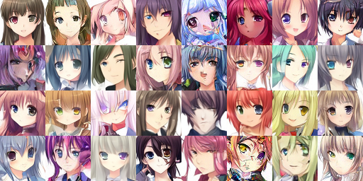
看一下结果如何：

感觉还不错，那么 DDIM 的学习到这里就告一段落了。

总结

感觉 DDIM 还是非常神奇的，通过改变推导方式去除了对马尔可夫假设的依赖，而且最后表达式中几个复杂的项相互都可以消掉，最后得到一个比较优美的结果。而且最重要的是采样速度真的变快了好多，也因此我直接把实验从集群上搬到了我自己的 PC 上，的确很高效。

本文的代码在如下的链接中，后续还会更新更多 diffusion models 相关的文章，欢迎追更：

• 完整代码：https://github.com/LittleNyima/code-snippets/tree/master/ddim-tutorial
• 模型权重：https://huggingface.co/LittleNyima/ddpm-anime-faces-64

参考资料：

1. diffusion model(二)：DDIM技术小结 (denoising diffusion implicit model)
2. 扩散模型（一）| DDPM & DDIM

本文原文以 CC BY-NC-SA 4.0 许可协议发布于 笔记｜扩散模型（二）：DDIM 理论与实现，转载请注明出处。