


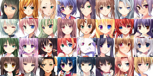
在正式开始之前先贴一个生成结果示例:
端午假期卷一卷,开一个新坑系统性地整理一下扩散模型的相关知识。扩散模型的名字来源于物理中的扩散过程,对于一张图像来说,类比扩散过程,向这张图像逐渐加入高斯噪声,当加入的次数足够多的时候,图像中像素的分布也会逐渐变成一个高斯分布。当然这个过程也可以反过来,如果我们设计一个神经网络,每次能够从图像中去掉一个高斯噪声,那么最后就能从一个高斯噪声得到一张图像。虽然一张有意义的图像不容易获得,但高斯噪声很容易采样,如果能实现这个逆过程,就能实现图像的生成。
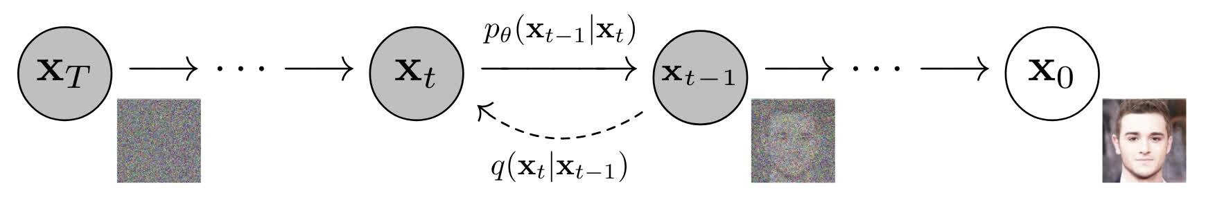
这个过程可以形象地用上图表示,扩散模型中有两个过程,分别是前向过程(从图像加噪得到噪音)和反向过程(从噪音去噪得到图像)。在上图中,向图像 x 0 \mathbf{x}_0 x0 逐渐添加噪声可以得到一系列的 x 1 , x 2 , . . . , x T \mathbf{x}_1,\mathbf{x}_2,...,\mathbf{x}_T x1,x2,...,xT,最后的 x T \mathbf{x}_T xT 即接近完全的高斯噪声,这个过程显然是比较容易的。而从 x T \mathbf{x}_T xT 逐渐去噪得到 x 0 \mathbf{x}_0 x0 并不容易,扩散模型学习的就是这个去噪的过程。
前向过程
我们从比较简单的前向过程开始,第一个问题是如何向图像中添加高斯噪声。在 DDPM 中,加噪的方式是直接对图像和标准高斯噪声
ϵ
t
−
1
∼
N
(
0
,
I
)
\epsilon_{t-1}\sim\mathcal{N}(0,\mathbf{I})
ϵt−1∼N(0,I) 进行加权求和:
x
t
=
1
−
β
t
x
t
−
1
+
β
t
ϵ
t
−
1
\mathbf{x}_{t}=\sqrt{1-\beta_t}\mathbf{x}_{t-1}+\sqrt{\beta_t}\epsilon_{t-1}
xt=1−βtxt−1+βtϵt−1
这里的
β
t
\beta_t
βt 就是每一步加噪使用的方差,在实际上进行加噪时,起始时使用的方差比较小,随着加噪步骤增加,方差会逐渐增大。例如在 DDPM 的原文中,使用的方差是从
β
1
=
1
0
−
4
\beta_1=10^{-4}
β1=10−4 随加噪时间步线性增大到
β
T
=
0.02
\beta_T=0.02
βT=0.02。这样设置主要是为了方便模型进行学习,如果在最开始就加入很大的噪声,对图像信息的破坏会比较严重,不利于模型学习图像的信息。这个过程也可以从反向进行理解,即去噪时先去掉比较大的噪音得到图像的雏形,再去掉小噪音进行细节的微调。
在上边的公式里,我们可以认为
x
t
\mathbf{x}_t
xt 满足均值为
1
−
β
t
x
t
−
1
\sqrt{1-\beta_t}\mathbf{x}_{t-1}
1−βtxt−1,方差为
β
t
I
\sqrt{\beta_t}\mathbf{I}
βtI 的高斯分布。这样可以把上述加权求和的过程写成条件概率分布的形式:
q
(
x
t
∣
x
t
−
1
)
=
N
(
x
t
;
1
−
β
t
x
t
−
1
,
β
t
I
)
q(\mathbf{x}_t|\mathbf{x}_{t-1})=\mathcal{N}(\mathbf{x}_t;\sqrt{1-\beta_t}\mathbf{x}_{t-1},\beta_t\mathbf{I})
q(xt∣xt−1)=N(xt;1−βtxt−1,βtI)
上边等号的右边表示的就是当前的变量
x
t
\mathbf{x}_t
xt 满足一个
N
(
1
−
β
t
x
t
−
1
,
β
t
I
)
\mathcal{N}(\sqrt{1-\beta_t}\mathbf{x}_{t-1},\beta_t\mathbf{I})
N(1−βtxt−1,βtI) 的概率分布。通过上边的公式我们可以看到,每一个时间步的
x
t
\mathbf{x}_t
xt 都只和
x
t
−
1
\mathbf{x}_{t-1}
xt−1 有关,因此这个扩散过程是一个马尔可夫过程。在前向过程中,每一步的
β
\beta
β 都是固定的,真正的变量只有
x
t
−
1
\mathbf{x}_{t-1}
xt−1,那么我们可以将公式中的
x
t
−
1
\mathbf{x}_{t-1}
xt−1 进一步展开:
x
t
=
1
−
β
t
x
t
−
1
+
β
t
ϵ
t
−
1
=
1
−
β
t
(
1
−
β
t
−
1
x
t
−
2
+
β
t
−
1
ϵ
t
−
2
)
+
β
t
ϵ
t
−
1
=
(
1
−
β
t
)
(
1
−
β
t
−
1
)
x
t
−
2
+
(
1
−
β
t
)
β
t
−
1
ϵ
t
−
2
+
β
t
ϵ
t
−
1
\begin{aligned} \mathbf{x}_t&=\sqrt{1-\beta_t}\mathbf{x}_{t-1}+\sqrt{\beta_t}\epsilon_{t-1}\\ &=\sqrt{1-\beta_t}(\sqrt{1-\beta_{t-1}}\mathbf{x}_{t-2}+\sqrt{\beta_{t-1}}\epsilon_{t-2})+\sqrt{\beta_t}\epsilon_{t-1}\\ &=\sqrt{(1-\beta_t)(1-\beta_{t-1})}\mathbf{x}_{t-2}+\sqrt{(1-\beta_t)\beta_{t-1}}\epsilon_{t-2}+\sqrt{\beta_t}\epsilon_{t-1} \end{aligned}
xt=1−βtxt−1+βtϵt−1=1−βt(1−βt−1xt−2+βt−1ϵt−2)+βtϵt−1=(1−βt)(1−βt−1)xt−2+(1−βt)βt−1ϵt−2+βtϵt−1
在上边的公式里,实际上
ϵ
t
−
2
\epsilon_{t-2}
ϵt−2 和
ϵ
t
−
1
\epsilon_{t-1}
ϵt−1 是同分布的,都是
N
(
0
,
1
)
\mathcal{N}(0,1)
N(0,1),因此可以进行合并:
x
t
=
(
1
−
β
t
)
(
1
−
β
t
−
1
)
x
t
−
2
+
(
(
1
−
β
t
)
β
t
−
1
)
2
+
(
β
t
)
2
ϵ
ˉ
t
−
2
=
(
1
−
β
t
)
(
1
−
β
t
−
1
)
x
t
−
2
+
1
−
(
1
−
β
t
)
(
1
−
β
t
−
1
)
ϵ
ˉ
t
−
2
\begin{aligned} \mathbf{x}_t&=\sqrt{(1-\beta_t)(1-\beta_{t-1})}\mathbf{x}_{t-2}+\sqrt{(\sqrt{(1-\beta_t)\beta_{t-1}})^2+(\sqrt{\beta_t})^2}\bar{\epsilon}_{t-2}\\ &=\sqrt{(1-\beta_t)(1-\beta_{t-1})}\mathbf{x}_{t-2}+\sqrt{1-(1-\beta_t)(1-\beta_{t-1})}\bar{\epsilon}_{t-2} \end{aligned}
xt=(1−βt)(1−βt−1)xt−2+((1−βt)βt−1)2+(βt)2ϵˉt−2=(1−βt)(1−βt−1)xt−2+1−(1−βt)(1−βt−1)ϵˉt−2
令
α
t
=
1
−
β
t
\alpha_t=1-\beta_t
αt=1−βt,
α
ˉ
t
=
∏
i
=
1
t
α
i
\bar{\alpha}_t=\prod_{i=1}^t\alpha_i
αˉt=∏i=1tαi,继续推导,可以得到:
x
t
=
α
t
α
t
−
1
x
t
−
2
+
1
−
α
t
α
t
−
1
ϵ
ˉ
t
−
2
=
⋯
=
α
ˉ
t
x
0
+
1
−
α
ˉ
t
ϵ
\begin{aligned} \mathbf{x}_t&=\sqrt{\alpha_t\alpha_{t-1}}\mathbf{x}_{t-2}+\sqrt{1-\alpha_t\alpha_{t-1}}\bar{\epsilon}_{t-2}\\ &=\cdots\\ &=\sqrt{\bar{\alpha}_t}\mathbf{x}_0+\sqrt{1-\bar{\alpha}_t}\epsilon \end{aligned}
xt=αtαt−1xt−2+1−αtαt−1ϵˉt−2=⋯=αˉtx0+1−αˉtϵ
通过上述的推导,我们发现给定
x
0
\mathbf{x}_0
x0 和加噪的时间步,可以直接用一步就得到
x
t
\mathbf{x}_t
xt,而并不需要一步步地重复最开始的加权求和。和上述同理,这个关系也可以写成:
q
(
x
t
∣
x
0
)
=
N
(
x
t
;
α
ˉ
t
x
0
,
(
1
−
α
ˉ
t
)
I
)
q(\mathbf{x}_t|\mathbf{x}_0)=\mathcal{N}(\mathbf{x}_t;\sqrt{\bar{\alpha}_t}\mathbf{x}_0,(1-\bar{\alpha}_t)\mathbf{I})
q(xt∣x0)=N(xt;αˉtx0,(1−αˉt)I)
从这个式子里我们可以看出,加噪过程中的
x
t
\mathbf{x}_t
xt 可以看作原始图像
x
0
\mathbf{x}_0
x0 和高斯噪声
ϵ
\epsilon
ϵ 的线性组合,且两个组合系数的平方和为 1。在实现加噪过程时,加噪的 scheduler 也是根据
α
ˉ
t
\bar{\alpha}_t
αˉt 设计的,这样更加直接,且为了保证最后得到的足够接近噪声,可以将
α
ˉ
t
\bar\alpha_t
αˉt 直接设置为一个接近 0 的数。
反向过程
正如文章开始所说的,反向过程就是从
x
T
\mathbf{x}_T
xT 逐渐去噪得到
x
0
\mathbf{x}_0
x0 的过程,也就是求
q
(
x
t
−
1
∣
x
t
)
q(\mathbf{x}_{t-1}|\mathbf{x}_t)
q(xt−1∣xt)。根据贝叶斯公式:
q
(
x
t
−
1
∣
x
t
)
=
q
(
x
t
∣
x
t
−
1
)
q
(
x
t
−
1
)
q
(
x
t
)
q(\mathbf{x}_{t-1}|\mathbf{x}_t)=\frac{q(\mathbf{x}_t|\mathbf{x}_{t-1})q(\mathbf{x}_{t-1})}{q(\mathbf{x}_t)}
q(xt−1∣xt)=q(xt)q(xt∣xt−1)q(xt−1)
在上边的公式里,在前文中我们已经给出了
q
(
x
∣
x
t
−
1
)
q(\mathbf{x}|\mathbf{x}_{t-1})
q(x∣xt−1),但
q
(
x
t
−
1
)
q(\mathbf{x}_{t-1})
q(xt−1) 和
q
(
x
t
)
q(\mathbf{x}_t)
q(xt) 依然是未知的。虽然这两个分布目前未知,但是在上一节的最后,我们已经推导出了
q
(
x
t
∣
x
0
)
q(\mathbf{x}_t|\mathbf{x}_0)
q(xt∣x0) 这个分布,那么我们可以给上面的贝叶斯公式加上
x
0
\mathbf{x}_0
x0 作为条件,将等号右侧的两个未知分布转化为已知分布:
q
(
x
t
−
1
∣
x
t
,
x
0
)
=
q
(
x
t
∣
x
t
−
1
,
x
0
)
q
(
x
t
−
1
∣
x
0
)
q
(
x
t
∣
x
0
)
q(\mathbf{x}_{t-1}|\mathbf{x}_t,\mathbf{x}_0)=\frac{q(\mathbf{x}_t|\mathbf{x}_{t-1},\mathbf{x}_0)q(\mathbf{x}_{t-1}|\mathbf{x}_0)}{q(\mathbf{x}_t|\mathbf{x}_0)}
q(xt−1∣xt,x0)=q(xt∣x0)q(xt∣xt−1,x0)q(xt−1∣x0)
而且因为先验分布
q
(
x
t
∣
x
t
−
1
)
q(\mathbf{x}_t|\mathbf{x}_{t-1})
q(xt∣xt−1) 是马尔可夫过程,
x
t
\mathbf{x}_t
xt 只与
x
t
−
1
\mathbf{x}_{t-1}
xt−1 有关,而与
x
0
\mathbf{x}_0
x0 无关,所以上边式子里的
q
(
x
t
∣
x
t
−
1
,
x
0
)
=
q
(
x
t
∣
x
t
−
1
)
q(\mathbf{x}_t|\mathbf{x}_{t-1},\mathbf{x}_0)=q(\mathbf{x}_t|\mathbf{x}_{t-1})
q(xt∣xt−1,x0)=q(xt∣xt−1)。但推导到这里还有问题,我们把
x
0
\mathbf{x}_0
x0 加入到了条件概率分布的条件中,但
x
0
\mathbf{x}_0
x0 依然是未知的,因此我们需要继续推导出一个与
x
0
\mathbf{x}_0
x0 无关的式子。
上面的公式右侧的几个条件概率分布全都是高斯分布:
q
(
x
t
∣
x
t
−
1
)
=
N
(
x
t
;
α
t
x
t
−
1
,
1
−
α
t
)
q
(
x
t
−
1
∣
x
0
)
=
N
(
x
t
−
1
;
α
ˉ
t
−
1
x
0
,
1
−
α
ˉ
t
−
1
)
q
(
x
t
∣
x
0
)
=
N
(
x
t
;
α
ˉ
t
x
0
,
1
−
α
ˉ
t
)
\begin{aligned} q(\mathbf{x}_t|\mathbf{x}_{t-1})&=\mathcal{N}(\mathbf{x}_t;\sqrt{\alpha_t}\mathbf{x}_{t-1},1-\alpha_t)\\ q(\mathbf{x}_{t-1}|\mathbf{x}_0)&=\mathcal{N}(\mathbf{x}_{t-1};\sqrt{\bar{\alpha}_{t-1}}\mathbf{x}_0,1-\bar{\alpha}_{t-1})\\ q(\mathbf{x}_t|\mathbf{x}_0)&=\mathcal{N}(\mathbf{x}_t;\sqrt{\bar{\alpha}_t}\mathbf{x}_0,1-\bar\alpha_t) \end{aligned}
q(xt∣xt−1)q(xt−1∣x0)q(xt∣x0)=N(xt;αtxt−1,1−αt)=N(xt−1;αˉt−1x0,1−αˉt−1)=N(xt;αˉtx0,1−αˉt)
用概率密度函数把这个公式展开,如果不看前边的常数项,可以得到:
q
(
x
t
−
1
∣
x
t
,
x
0
)
∝
exp
(
−
1
2
[
(
x
t
−
α
t
x
t
−
1
)
2
β
t
+
(
x
t
−
1
−
α
ˉ
t
−
1
x
0
)
2
1
−
α
ˉ
t
−
1
+
(
x
t
−
α
ˉ
t
x
0
)
1
−
α
ˉ
t
]
)
\begin{aligned} q(\mathbf{x}_{t-1}|\mathbf{x}_t,\mathbf{x}_0)&\propto\exp\left(-\frac{1}{2}\left[\frac{(\mathbf{x}_t-\sqrt{\alpha_t}\mathbf{x}_{t-1})^2}{\beta_t}+\frac{(\mathbf{x}_{t-1}-\sqrt{\bar\alpha_{t-1}}\mathbf{x}_0)^2}{1-\bar\alpha_{t-1}}+\frac{(\mathbf{x}_t-\sqrt{\bar{\alpha}_t}\mathbf{x}_0)}{1-\bar\alpha_t}\right]\right)\\ \end{aligned}
q(xt−1∣xt,x0)∝exp(−21[βt(xt−αtxt−1)2+1−αˉt−1(xt−1−αˉt−1x0)2+1−αˉt(xt−αˉtx0)])
因为我们在这一步去噪的时候想求得的是
x
t
−
1
\mathbf{x}_{t-1}
xt−1 的分布,所以我们把上式展开并整理成一个关于
x
t
−
1
\mathbf{x}_{t-1}
xt−1 的多项式:
q
(
x
t
−
1
∣
x
t
,
x
0
)
∝
exp
(
−
1
2
[
(
α
t
β
t
+
1
1
−
α
ˉ
t
−
1
)
x
t
−
1
2
−
(
2
α
t
β
t
x
t
+
2
α
ˉ
t
−
1
1
−
α
ˉ
t
−
1
x
0
)
x
t
−
1
+
C
(
x
t
,
x
0
)
]
)
q(\mathbf{x}_{t-1}|\mathbf{x}_t,\mathbf{x}_0)\propto\exp\left(-\frac{1}{2}\left[\left(\frac{\alpha_t}{\beta_t}+\frac{1}{1-\bar\alpha_{t-1}}\right)\mathbf{x}_{t-1}^2-\left(\frac{2\sqrt{\alpha_t}}{\beta_t}\mathbf{x}_t+\frac{2\sqrt{\bar\alpha_{t-1}}}{1-\bar\alpha_{t-1}}\mathbf{x}_0\right)\mathbf{x}_{t-1}+C(\mathbf{x}_t,\mathbf{x}_0)\right]\right)
q(xt−1∣xt,x0)∝exp(−21[(βtαt+1−αˉt−11)xt−12−(βt2αtxt+1−αˉt−12αˉt−1x0)xt−1+C(xt,x0)])
上边的式子里常数项不重要(因为可以直接变成常数从指数部分挪走),所以可以暂时不管。对比高斯分布(可以证明反向过程的分布也是高斯分布)的指数部分
exp
(
−
1
2
(
1
σ
2
x
2
−
2
μ
σ
2
x
+
μ
2
σ
2
)
)
\exp\left(-\frac{1}{2}\left(\frac{1}{\sigma^2}x^2-\frac{2\mu}{\sigma^2}x+\frac{\mu^2}{\sigma^2}\right)\right)
exp(−21(σ21x2−σ22μx+σ2μ2)):
{
1
σ
2
=
α
t
β
t
+
1
1
−
α
ˉ
t
−
1
2
μ
σ
2
=
2
α
t
β
t
x
t
+
2
α
ˉ
t
−
1
1
−
α
ˉ
t
−
1
x
0
\begin{cases} \begin{aligned} \frac{1}{\sigma^2}&=\frac{\alpha_t}{\beta_t}+\frac{1}{1-\bar\alpha_{t-1}}\\ \frac{2\mu}{\sigma^2}&=\frac{2\sqrt{\alpha_t}}{\beta_t}\mathbf{x}_t+\frac{2\sqrt{\bar\alpha_{t-1}}}{1-\bar\alpha_{t-1}}\mathbf{x}_0 \end{aligned} \end{cases}
⎩
⎨
⎧σ21σ22μ=βtαt+1−αˉt−11=βt2αtxt+1−αˉt−12αˉt−1x0
可以发现
σ
\sigma
σ 的表达式里都是我们 scheduler 里的定值,而求解出均值
μ
\mu
μ:
μ
=
α
t
(
1
−
α
ˉ
t
−
1
)
1
−
α
ˉ
t
x
t
+
α
ˉ
t
−
1
β
t
1
−
α
ˉ
t
x
0
\mu=\frac{\sqrt{\alpha_t}(1-\bar\alpha_{t-1})}{1-\bar\alpha_t}\mathbf{x}_t+\frac{\sqrt{\bar\alpha_{t-1}}\beta_t}{1-\bar\alpha_t}\mathbf{x}_0
μ=1−αˉtαt(1−αˉt−1)xt+1−αˉtαˉt−1βtx0
代入上一章最后的
x
t
=
α
ˉ
t
x
0
+
1
−
α
ˉ
t
ϵ
\mathbf{x}_t=\sqrt{\bar{\alpha}_t}\mathbf{x}_0+\sqrt{1-\bar{\alpha}_t}\epsilon
xt=αˉtx0+1−αˉtϵ,得到:
μ
=
1
α
t
(
x
t
−
1
−
α
t
1
−
α
ˉ
t
ϵ
~
t
)
\mu=\frac{1}{\sqrt{\alpha_t}}\left(\mathbf{x}_t-\frac{1-\alpha_t}{\sqrt{1-\bar\alpha_t}}\tilde{\epsilon}_t\right)
μ=αt1(xt−1−αˉt1−αtϵ~t)
注意在反向过程中我们并不知道在前向过程中加入的噪声
ϵ
t
\epsilon_t
ϵt 是
N
(
0
,
1
)
\mathcal{N}(0,1)
N(0,1) 中的具体哪一个噪声,而噪声也没有办法继续转换成其他的形式。因此我们使用神经网络在反向过程中估计的目标就是
ϵ
~
t
\tilde{\epsilon}_t
ϵ~t。在这个网络中,输入除了
x
t
\mathbf{x}_t
xt 之外还需要
t
t
t,可以简单理解为:加噪过程中
x
t
\mathbf{x}_t
xt 的噪声含量是由
t
t
t 决定的,因此在预测噪声时也需要知道时间步
t
t
t 作为参考,以降低预测噪声的难度。
注:关于反向过程为什么要这样做,Lilian Weng 基于变分推断给出了一个复杂的证明,因为过于难以理解,这里暂且把它跳过。(以后有可能会填坑,也有可能不会x)
具体的训练过程
我们已经知道了去噪网络的参数和预测目标,下一个问题就是如何去训练这个去噪网络。原始论文中给出了如下的训练过程:
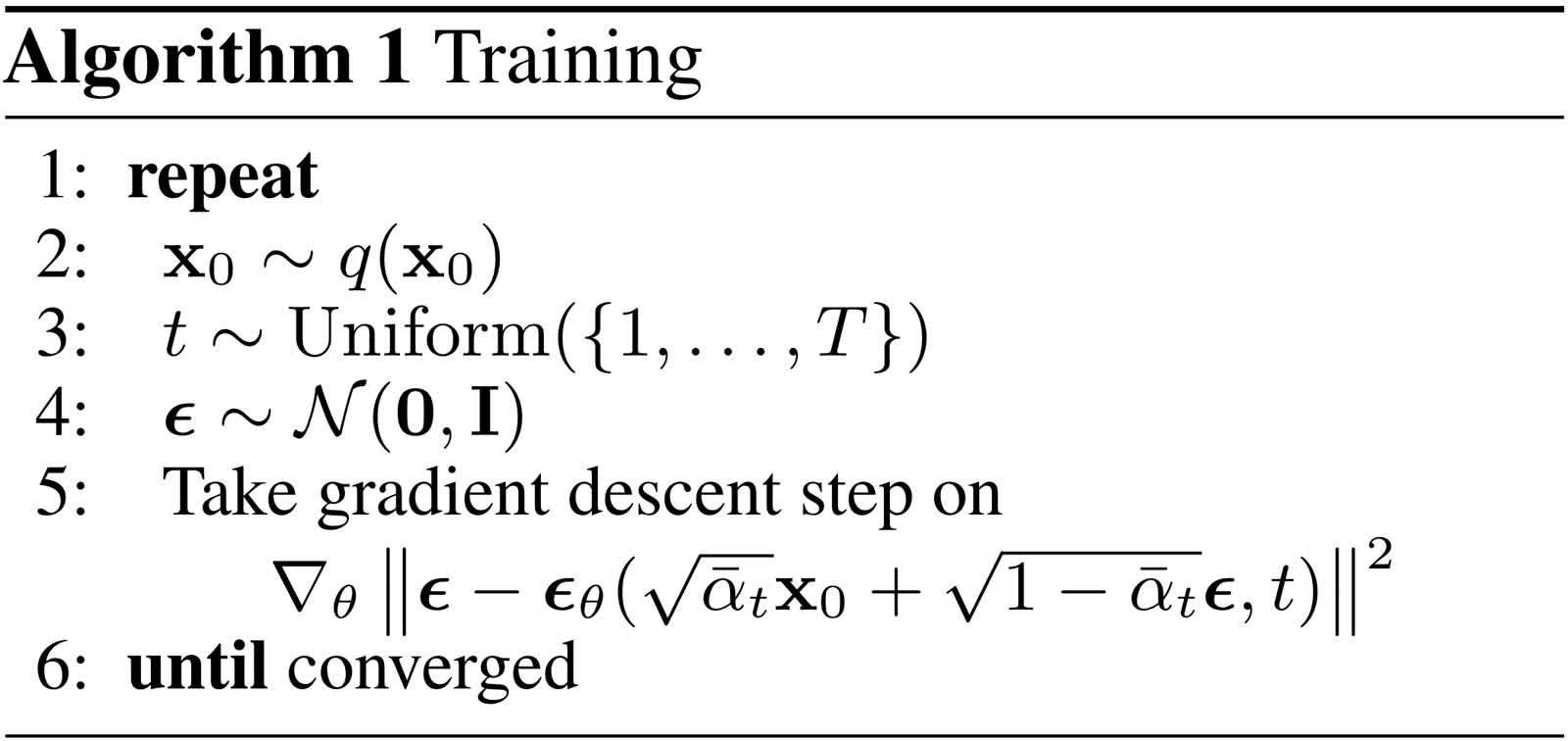
在上面的算法中,首先从数据集 q ( x 0 ) q(\mathbf{x}_0) q(x0) 中采样出 x 0 \mathbf{x}_0 x0,从 1 到 T 的均匀分布中采样出 t t t,从标准高斯分布中采样出 ϵ \epsilon ϵ。然后根据 x t = α ˉ t x 0 + 1 − α ˉ t ϵ \mathbf{x}_t=\sqrt{\bar{\alpha}_t}\mathbf{x}_0+\sqrt{1-\bar{\alpha}_t}\epsilon xt=αˉtx0+1−αˉtϵ 将 x 0 \mathbf{x}_0 x0 与 ϵ \epsilon ϵ 加权求和得到噪声图,最后将噪声图和时间步输入到网络中预测噪声,并用真实的噪声计算出 L2 损失进行优化。
这里比较难理解的是 ϵ \epsilon ϵ 本身就是从标准高斯分布中采样出的,为什么还需要一个网络专门对其进行预测。我个人的理解是:尽管每次添加的噪声都是从固定的分布中采样出的,但如果用同一个分布中的另一个采样出的样本将其代替,就会向去噪过程引入一定的误差,最后这些误差积累的结果会破坏最终生成的图像。
具体的采样过程
论文中同样也给出了采样过程:
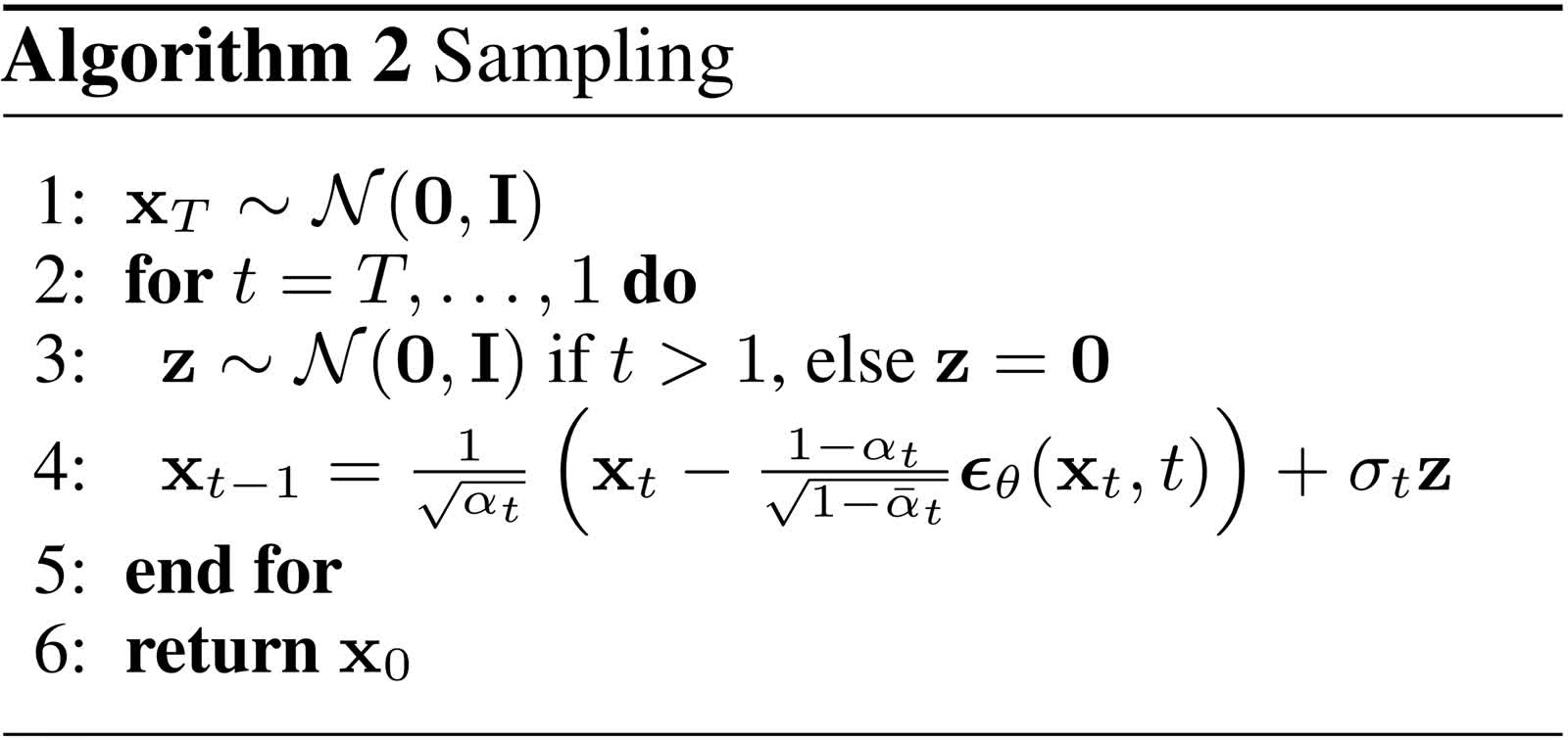
具体来说,首先从标准正态分布中采样出
x
T
\mathbf{x}_T
xT 作为初始的图像,然后重复
T
T
T 步去噪过程。在每一步去噪过程中,由于我们已经推导出:
q
(
x
t
−
1
∣
x
t
)
=
N
(
x
t
−
1
;
1
α
t
(
x
t
−
1
−
α
t
1
−
α
ˉ
t
ϵ
~
t
)
,
σ
t
2
)
q(\mathbf{x}_{t-1}|\mathbf{x}_t)=\mathcal{N}\left(\mathbf{x}_{t-1};\frac{1}{\sqrt{\alpha_t}}\left(\mathbf{x}_t-\frac{1-\alpha_t}{\sqrt{1-\bar\alpha_t}}\tilde{\epsilon}_t\right),\sigma_t^2\right)
q(xt−1∣xt)=N(xt−1;αt1(xt−1−αˉt1−αtϵ~t),σt2)
利用一个重参数化技巧:从
N
(
μ
,
σ
2
)
\mathcal{N}(\mu,\sigma^2)
N(μ,σ2) 采样可以实现为从
N
(
0
,
1
)
\mathcal{N}(0,1)
N(0,1) 采样出
ϵ
\epsilon
ϵ,再计算
μ
+
ϵ
⋅
σ
\mu+\epsilon\cdot\sigma
μ+ϵ⋅σ。这样即可实现从上述的高斯分布中采样出
x
t
−
1
\mathbf{x}_{t-1}
xt−1。如此重复
T
T
T 次即可得到最终的结果,注意最后一步的时候没有采样,而是只加上了均值。
DDPM 的代码实现
现有的主流方法使用 UNet 来实现去噪网络,如下图所示。
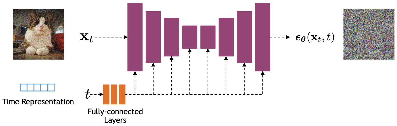
为了降低理解的难度,我们这里不关心这个去噪网络的具体实现,只需要知道这个网络接收一个噪声图
x
t
\mathbf{x}_t
xt 和一个时间步
t
t
t 作为参数,并输出一个噪声的预测结果
ϵ
θ
(
x
t
,
t
)
\epsilon_\theta(\mathbf{x}_t,t)
ϵθ(xt,t)。在 diffusers 库中已经实现了一个 2D UNet 网络,我们直接使用即可。下面我们也主要使用 diffusers 实现 DDPM 模型。
训练参数
首先配置训练的参数:
from dataclasses import dataclass

@dataclass
class TrainingConfig:
    image_size = 64
    train_batch_size = 16
    eval_batch_size = 16
    num_epochs = 50
    gradient_accumulation_steps = 1
    learning_rate = 1e-4
    lr_warmup_steps = 500
    mixed_precision = "fp16"
    output_dir = "ddpm-animefaces-64"
    overwrite_output_dir = True

config = TrainingConfig()
训练数据
我们使用 huggan/anime-faces 数据集,这个数据集由 21551 张分辨率为 64x64 的动漫人物头像组成。我们加载这个数据集:
from datasets import load_dataset

dataset = load_dataset("huggan/anime-faces", split="train")
dataset = dataset.select(range(21551))
由于这个数据集的作者组织数据的方式不太规范,所以最后加载进来实际上数据集的长度是 86204,也就是 21551 张图片每张重复了 4 次,我们只需要保留前 21551 个样本即可。
然后为数据集设置预处理函数:
from torchvision import transforms

def get_transform():
    preprocess = transforms.Compose([
        transforms.Resize(config.image_size),
        transforms.ToTensor(),
        transforms.Normalize([0.5], [0.5]),
    ])
    def transform(samples):
        images = [preprocess(img.convert("RGB")) for img in samples["image"]]
        return dict(images=images)
    return transform

dataset.set_transform(get_transform())
最后创建 dataloader:
from torch.utils.data import DataLoader

dataloader = DataLoader(dataset, batch_size=config.train_batch_size, shuffle=True)
降噪网络
我们可以直接用 diffusers 创建降噪网络:
from diffusers import UNet2DModel

model = UNet2DModel(
    sample_size=config.image_size,
    in_channels=3,
    out_channels=3,
    layers_per_block=2,
    block_out_channels=(128, 128, 256, 256, 512, 512),
    down_block_types=(
        "DownBlock2D",
        "DownBlock2D",
        "DownBlock2D",
        "DownBlock2D",
        "AttnDownBlock2D",
        "DownBlock2D",
    ),
    up_block_types=(
        "UpBlock2D",
        "AttnUpBlock2D",
        "UpBlock2D",
        "UpBlock2D",
        "UpBlock2D",
        "UpBlock2D",
    ),
)
核心代码
前边的三个部分分别配置了一些训练参数,以及训练数据和模型,这些都是比较工程化的部分,而我们在上面推导的 DDPM 核心算法还没有实现。在这一小节我们主要来实现核心的算法。
首先我们需要先定义 β \beta β、 α \alpha α,以及 α ˉ \bar\alpha αˉ 等最基本的常量,这里我们保持 DDPM 原论文的配置,也就是 β \beta β 初始为 1 × 1 0 − 4 1\times10^{-4} 1×10⁻⁴,最终为 0.02 0.02 0.02,且共有 1000 1000 1000 个时间步:
import torch

class DDPM:
    def __init__(
        self,
        num_train_timesteps:int = 1000,
        beta_start: float = 0.0001,
        beta_end: float = 0.02,
    ):
        self.betas = torch.linspace(beta_start, beta_end, num_train_timesteps, dtype=torch.float32)
        self.alphas = 1.0 - self.betas
        self.alphas_cumprod = torch.cumprod(self.alphas, dim=0)
        self.timesteps = torch.arange(num_train_timesteps - 1, -1, -1)
然后是比较简单的前向过程,只需要实现加噪即可,按照 x t = α ˉ t x 0 + 1 − α ˉ t ϵ \mathbf{x}_t=\sqrt{\bar{\alpha}_t}\mathbf{x}_0+\sqrt{1-\bar{\alpha}_t}\epsilon xt=αˉtx0+1−αˉtϵ 这个公式实现即可。注意需要将系数的维度数量都与输入样本对齐:
class DDPM:
    ...

    def add_noise(
        self,
        original_samples: torch.Tensor,
        noise: torch.Tensor,
        timesteps: torch.Tensor,
    ):
        alphas_cumprod = self.alphas_cumprod.to(device=original_samples.device ,dtype=original_samples.dtype)
        noise = noise.to(original_samples.device)
        timesteps = timesteps.to(original_samples.device)

        # \sqrt{\bar\alpha_t}
        sqrt_alpha_prod = alphas_cumprod[timesteps].flatten() ** 0.5
        while len(sqrt_alpha_prod.shape) < len(original_samples.shape):
            sqrt_alpha_prod = sqrt_alpha_prod.unsqueeze(-1)

        # \sqrt{1 - \bar\alpha_t}
        sqrt_one_minus_alpha_prod = (1.0 - alphas_cumprod[timesteps]).flatten() ** 0.5
        while len(sqrt_one_minus_alpha_prod.shape) < len(original_samples.shape):
            sqrt_one_minus_alpha_prod = sqrt_one_minus_alpha_prod.unsqueeze(-1)

        return sqrt_alpha_prod * original_samples + sqrt_one_minus_alpha_prod * noise
反向过程相对来说比较复杂,不过因为我们已经完成了公式的推导,只需要按照公式实现即可。我们也再把公式贴到这里,对着公式实现具体的代码:
σ
=
(
α
t
β
t
+
1
1
−
α
ˉ
t
−
1
)
−
1
/
2
μ
=
1
α
t
(
x
t
−
1
−
α
t
1
−
α
ˉ
t
ϵ
~
t
)
\begin{aligned} \sigma&=\left(\frac{\alpha_t}{\beta_t}+\frac{1}{1-\bar\alpha_{t-1}}\right)^{-1/2}\\ \mu&=\frac{1}{\sqrt{\alpha_t}}\left(\mathbf{x}_t-\frac{1-\alpha_t}{\sqrt{1-\bar\alpha_t}}\tilde{\epsilon}_t\right) \end{aligned}
σμ=(βtαt+1−αˉt−11)−1/2=αt1(xt−1−αˉt1−αtϵ~t)
class DDPM:
    ...

    @torch.no_grad()
    def sample(
        self,
        unet: UNet2DModel,
        batch_size: int,
        in_channels: int,
        sample_size: int,
    ):
        betas = self.betas.to(unet.device)
        alphas = self.alphas.to(unet.device)
        alphas_cumprod = self.alphas_cumprod.to(unet.device)
        timesteps = self.timesteps.to(unet.device)
        images = torch.randn((batch_size, in_channels, sample_size, sample_size), device=unet.device)
        for timestep in tqdm(timesteps, desc='Sampling'):
            pred_noise: torch.Tensor = unet(images, timestep).sample

            # mean of q(x_{t-1}|x_t)
            alpha_t = alphas[timestep]
            alpha_cumprod_t = alphas_cumprod[timestep]
            sqrt_alpha_t = alpha_t ** 0.5
            one_minus_alpha_t = 1.0 - alpha_t
            sqrt_one_minus_alpha_cumprod_t = (1 - alpha_cumprod_t) ** 0.5
            mean = (images - one_minus_alpha_t / sqrt_one_minus_alpha_cumprod_t * pred_noise) / sqrt_alpha_t

            # variance of q(x_{t-1}|x_t)
            if timestep > 0:
                beta_t = betas[timestep]
                one_minus_alpha_cumprod_t_minus_one = 1.0 - alphas_cumprod[timestep - 1]
                one_divided_by_sigma_square = alpha_t / beta_t + 1.0 / one_minus_alpha_cumprod_t_minus_one
                variance = (1.0 / one_divided_by_sigma_square) ** 0.5
            else:
                variance = torch.zeros_like(timestep)

            epsilon = torch.randn_like(images)
            images = mean + variance * epsilon
        images = (images / 2.0 + 0.5).clamp(0, 1).cpu().permute(0, 2, 3, 1).numpy()
        return images
训练与推理
最后是训练和推理的代码,这部分也比较工程,直接套用现成代码即可:
from accelerate import Accelerator
from diffusers.optimization import get_cosine_schedule_with_warmup
from diffusers.utils import make_image_grid, numpy_to_pil
import torch.nn.functional as F
import os

model = model.cuda()
ddpm = DDPM()
optimizer = torch.optim.AdamW(model.parameters(), lr=config.learning_rate)
lr_scheduler = get_cosine_schedule_with_warmup(
    optimizer=optimizer,
    num_warmup_steps=config.lr_warmup_steps,
    num_training_steps=(len(dataloader) * config.num_epochs),
)
accelerator = Accelerator(
    mixed_precision=config.mixed_precision,
    gradient_accumulation_steps=config.gradient_accumulation_steps,
    log_with="tensorboard",
    project_dir=os.path.join(config.output_dir, "logs"),
)
model, optimizer, dataloader, lr_scheduler = accelerator.prepare(
    model, optimizer, dataloader, lr_scheduler
)
global_step = 0
for epoch in range(config.num_epochs):
    progress_bar = tqdm(total=len(dataloader), disable=not accelerator.is_local_main_process, desc=f'Epoch {epoch}')

    for step, batch in enumerate(dataloader):
        clean_images = batch["images"]
        # Sample noise to add to the images
        noise = torch.randn(clean_images.shape, device=clean_images.device)
        bs = clean_images.shape[0]
        # Sample a random timestep for each image
        timesteps = torch.randint(
            0, ddpm.num_train_timesteps, (bs,), device=clean_images.device,
            dtype=torch.int64
        )
        # Add noise to the clean images according to the noise magnitude at each timestep
        noisy_images = ddpm.add_noise(clean_images, noise, timesteps)
        with accelerator.accumulate(model):
            # Predict the noise residual
            noise_pred = model(noisy_images, timesteps, return_dict=False)[0]
            loss = F.mse_loss(noise_pred, noise)
            accelerator.backward(loss)
            accelerator.clip_grad_norm_(model.parameters(), 1.0)
            optimizer.step()
            lr_scheduler.step()
            optimizer.zero_grad()
        progress_bar.update(1)
        logs = {"loss": loss.detach().item(), "lr": lr_scheduler.get_last_lr()[0], "step": global_step}
        progress_bar.set_postfix(**logs)
        accelerator.log(logs, step=global_step)
        global_step += 1

    if accelerator.is_main_process:
        # evaluate
        images = ddpm.sample(model, config.eval_batch_size, 3, config.image_size)
        image_grid = make_image_grid(numpy_to_pil(images), rows=4, cols=4)
        samples_dir = os.path.join(config.output_dir, 'samples')
        os.makedirs(samples_dir, exist_ok=True)
        image_grid.save(os.path.join(samples_dir, f'{global_step}.png'))
        # save models
        model.save_pretrained(config.output_dir)
结果展示
训练在一张 NVIDIA GeForce RTX 4090 GPU 上大概需要运行 3 个多小时,最后的结果大概长这个样子:
可以看到虽然里边难免有一些比较奇形怪状的结果,不过总体上来说已经初具雏形了。
总结
本文总结了 DDPM 的理论和实现方式,在代码部分我们是完全根据推导出的公式实现的采样过程。实际上在很多代码库中,采样过程并没有严格按照论文中的公式实现,而是先从 x t \mathbf{x}_t xt、 t t t 和预测的噪声反向计算出 x 0 \mathbf{x}_0 x0,再基于 μ = α t ( 1 − α ˉ t − 1 ) 1 − α ˉ t x t + α ˉ t − 1 β t 1 − α ˉ t x 0 \mu=\frac{\sqrt{\alpha_t}(1-\bar\alpha_{t-1})}{1-\bar\alpha_t}\mathbf{x}_t+\frac{\sqrt{\bar\alpha_{t-1}}\beta_t}{1-\bar\alpha_t}\mathbf{x}_0 μ=1−αˉtαt(1−αˉt−1)xt+1−αˉtαˉt−1βtx0 计算均值,这样的好处在于可以对 x 0 \mathbf{x}_0 x0 进一步规范化,控制输出的范围。
可以看出 DDPM 虽然理论比较复杂,但实现起来还是比较简单直接的。因为作者本人对 diffusion models 的理解也不算非常深入,所以如果文章有问题的话欢迎各位读者来讨论,后续(如果没有鸽掉的话)还会更新一些其他的 diffusion models 的文章,欢迎追更)
本文完整的代码以及训练好的模型见如下链接:
- 完整代码:https://github.com/LittleNyima/code-snippets/tree/master/ddpm-tutorial
- 模型权重:https://huggingface.co/LittleNyima/ddpm-anime-faces-64
参考资料:
本文原文以 CC BY-NC-SA 4.0 许可协议发布于 笔记|扩散模型(一):DDPM 理论与实现,转载请注明出处。


 765
765

 被折叠的 条评论
为什么被折叠?
被折叠的 条评论
为什么被折叠?
 到【灌水乐园】发言


