Wireless Communications - 2.4 Ray Tracing

提示：文章写完后，目录可以自动生成，如何生成可参考右边的帮助文档

---

Received Signal

Consider a signal transmitted through free space to a receiver located at distance d from the transmitter. Assume there are no obstructions between the transmitter and receiver. The channel model associated with this transmission is called a Line-Of-Sight (LOS) channel, and the corresponding received signal is called the LOS signal or ray. Free-space path loss introduces a complex scale factor, resulting in the received signal:
$$r(t)=\Re \left\{\frac{\lambda \sqrt{G_l}{e}^{-j(2\pi d/\lambda )}}{4\pi d}u(t)e^{j2\pi f_{c}t}\right\},$$ where $\sqrt{G_l}$ is the product of the transmit and receive antenna Field Radiation Patterns (FRP, 场辐射图) in the LOS direction, and the phase shift $e^{-j(2\pi d/\lambda )}$ ($e^{-j(2\pi f_c\tau }$, where delay $\tau =d/c$) is due to the distance $d$ the wave travels.

---

Preface

• In a typical urban or indoor environment, a radio signal transmitted from a fixed source will encounter multiple objects in the environment that produce reflected, diffracted, or scattered copies of the transmitted signal, as shown in the following figure.

• These additional copies of the transmitted, called multiple signal components, can be attenuated in power, delayed in time, and shifted in phase and/or frequency from the LOS signal path at the receiver.

• The 1) multipath and 2) transmitted signal are summed together at the receiver, which often produces distortion in the received signal.

---

Two-Ray Model

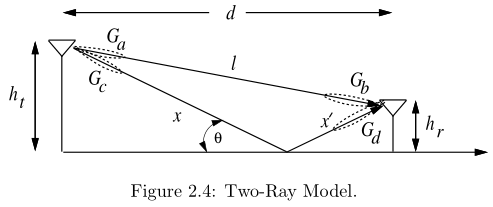
• The two-ray model is used when a single ground reflection dominates the multipath effect, as illustrated in Figure 2.4.
• The received signal consists of two components: 1) the LOS component or ray, which is just the transmitted signal propagating through free space, and 2) a reflected component or ray, which is the transmitted signal reflected off the ground.

The received LOS ray is given by the free-space propagation loss formulation r ( t ) = { λ G l e − j ( 2 π d / λ ) 4 π d u ( t ) e j 2 π f c t } r(t) = \{ \frac{\lambda \sqrt{G_l} e^{-j(2\pi d / \lambda)}}{4 \pi d} u(t) e^{j 2 \pi f_c t } \} r(t)={4πdλGl​ ​e−j(2πd/λ)​u(t)ej2πfc​t}.

The reflected ray is shown in Figure $2.4$ by the segments $x$ and $x^{\prime }$. If we ignore the effect of surface wave attenuation then, by superposition, the received signal for the two-ray model is $$r_{2ray}(t)=\Re \left\{\frac{\lambda }{4\pi }\left[\frac{\sqrt{G_l}u(t)e^{-j(2\pi l/\lambda )}}{l}+\frac{R\sqrt{G_r}u(t-\tau )e^{-j2\pi (x+x^{\prime })/\lambda }}{x+x^{\prime }}\right]e^{j(2\pi f_{c}t+{\varphi }_0)}\right\}.$$ where $x+x^{\prime }-l$ is the time delay of the ground reflection relative to the LOS ray, $\sqrt{G_l}=\sqrt{G_a{G}_b}$ is the product of transmit and receive antenna field radiation patterns in the LOS direction, $R$ is the ground reflection coefficient, and $\sqrt{G_r}=\sqrt{G_c{G}_d}$ is the product of transmit and receive antenna field radiation patterns corresponding to the rays of length $x$ and $x^{\prime }$, respectively. The delay spread of the two-ray model equals the delay between the LOS ray and reflected ray: $(x+x^{\prime }-l)/c$.

If the transmitted signal is narrowband relative to the delay spread $(\tau <<B_u^{-1})$, then $u(t)\approx u(t-\tau )$. Thus, the received power of the two-ray model for narrowband transmission is $$P_r=P_t{\left[\frac{\lambda }{4\pi }\right]}^2{\left|\frac{\sqrt{G_l}}{l}+\frac{R\sqrt{G_r}{e}^{-j\Delta \varphi }}{x+x^{\prime }}\right|}^2,(2.12)$$ where $△\varphi =2\pi (x+x^{\prime }-l)/\lambda$ is the phase difference between the two received signal components. The above equation has been shown to agree very closely with empirical data. If $d$ donotes the horizontal separation of the antennas, $h_t$ denotes the transmitter height, and $h_r$ denotes the receiver height, then using geometry we can show that $$x+x^{\prime }-l=\sqrt{(h_t+h_r{)}^2+d^2}-\sqrt{(h_t-h_r{)}^2+d^2}.$$

When $d$ is very large compared to $h_t+h_r$, we use a Taylor series approximation in the above equation to get $$△\varphi =\frac{2\pi (x+x^{\prime }-l)}{\lambda }\approx \frac{4\pi h_t{h}_r}{\lambda d}$$

The ground reflection coefficient is given by $$R=\frac{\sin \theta -Z}{\sin \theta +Z}(2.15)$$ where $$Z=\{\begin{array}{l}\sqrt{{ϵ}_r-{\cos }^2\theta }/{ϵ}_r\text{ for vertical polarization}\\ \sqrt{{ϵ}_r-{\cos }^2\theta }\text{ for horizontal polarization}\end{array}$$ and ${ϵ}_r$ is the dielectric constant of the ground.

We see from Figure 2.4 and (2.15) that for asymptotically large $d$, $x+x^{\prime }\approx l\approx d$, $\theta \approx 0$, $G_l\approx G_r$, and $R\approx -1$. Substituting these approximations into (2.12) yields that, in this asymptotic limit, the received signal power is approximately $$P_r\approx {\left[\frac{\lambda \sqrt{G_l}}{4\pi d}\right]}^2{\left[\frac{4\pi h_t{h}_r}{d^2}\right]}^2{P}_t$$, or equivalently, the $\mathbf{d}\mathbf{B}$ attenuation is given by
$$P_r(\text{dBm})=P_t(\text{dBm})+10lo{g}_{10}(G_l)+20lo{g}_{10}(h_t{h}_r)-40lo{g}_{10}(d).(2.18)$$ Thus, in the limit of asymptotically large $d$, the received power falls off inversely with the fourth power of $d$ and is independent of the wavelangth $\lambda$.

---

Discussion for the relationship of Distances and Received Power

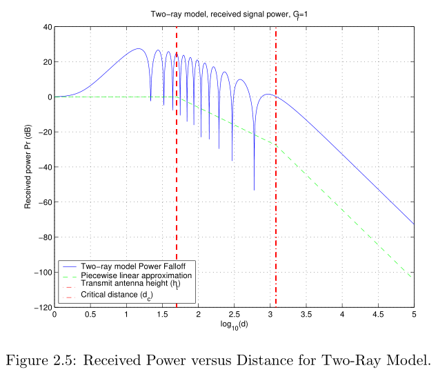
A plot of (2.18) as a function of distance is illustrated in Figure 2.5 for $f=900\text{MHz}$, $R=-1$, $h_t=50\text{m}$, $h_r=2m$, $G_l=1$, $G_r=1$, and transmit power normalized so that the plot starts at $0\text{dBm}$. This plot can be separated into three segments.

• For small distances $d<h_t$, the path loss is roughly flat and proportional to $\frac{1}{(d^2+h_t^2)}$, since, at these small distances, the distance between the transmitter and receiver is $D=\sqrt{d^2+(h_t-h_r{)}^2}$ and thus $\frac{1}{D^2}\approx \frac{1}{(d^2+h_t^2)}$ for $h_t>>h_r$, which is typically the case.
• For distances bigger than $h_t$ and up to a certain critical distance $d_c$, the wave experiences constructive and destructive interference of the two rays, resulting in a wave pattern with a sequence of maxima and minima. These maxima and minima are also refered to small scale loss or multipath fading.
• At the critical distance $d_c$, the final maxima is reached, after which the signal power falls off proportionally to $d^{-4}$.

The Properties of the Three Segments:

• In this first segment, power falloff is constant and proportional to $\frac{1}{d^2+h_t^2}$ ;
• For distance between $h_t$ and $d_c$, power falls off at $-20$ $\text{dB}$/decade ;
• At the distances greater than $d_c$, power falls off at $-40$ $\text{dB}$/decade.

---

Critical Distance for System Design

The critical distance can be used for system design.

For example, if propagation in a cellular system obeys the two-ray model, then the critical distance would be a natural size for the cell radius, since the path los associated with the interference outside the cell would be much larger than path loss for desired signals inside the cell. However, setting the cell radius to $d_c$ could result in very large cells.

Since smaller cells are more desirable, both to increase capacity and reduce transmit power, cell radii are typically much smaller than $d_c$.

Thus, with a two-ray propagation model, power falloff within these relatively small cells goes as distance squared. Moreover, propagation in cellular system rarely follows a two-ray model, since cancellation by reflected rays rarely occurs in all directions.

Example 2.2: Determine the critical distance for the two-ray model in an urban microcell ($h_t=10\text{m}$, $h_r=3\text{m}$) and an indoor microcell ($h_t=3\text{m},h_r=2\text{m}$) for $f_c=2\text{GHz}$.

Solution:
urban microcell: $$d_c=\frac{4h_t{h}_r}{\lambda }=800\text{m}$$
indoor microcell: $$d_c=\frac{4h_t{h}_r}{\lambda }=160\text{m}$$

Discussions:
A cell radius of 800 m in an urban microcell system is a bit large, and usually the radius is 100 m to maintain large capacity. However, if we used a cell size of 800 m under these system parameters, signal power would fall off as $d^2$ inside the cell, and interference from neighboring cells would fall off as $d^4$, and thus would be greatly reduced. Since these are many wall in indoor environments, an indoor system would typically have a smaller cell radius, on the order of 10-20 m.

---

Dielectric Canyon (Ten-Ray Model)

Assumptions

• This model assumes rectilinear streets with buildings along both sides of the street and transmitter and receiver antenna heights that are well below the tops of the buildings.
• The building-lined streets acts as a dielectric canyon to the propagating signal.
• Theoretically, an infinite number of rays can be reflected off the building fronts to arrive at the receiver. And, singal paths corresponding to more than three reflections can generally be ignored due their large energy dissipation.

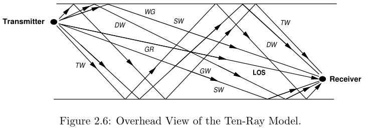
As shown in the following figure, the ten rays incorporate all paths with one, two, or three reflections:

• the LOS path;
• the ground reflected (GR) path;
• the single-wall (SW), the double-wall (DW), the triple-wall paths;
• the wall-ground (WG), and ground-wall (GW) reflected paths.

---

Received Signal

For this model, the received signal is given by
$$r_{10ray}(t)=\Re \left\{\frac{\lambda }{4\pi }\left[\frac{\sqrt{G_l}u(t)e^{-j(2\pi l)/\lambda }}{l}+\sum _{i=1}^9\frac{R_i\sqrt{G_{x_i}}u\left(t-{\tau }_i\right)e^{-j\left(2\pi x_i\right)/\lambda }}{x_i}\right]e^{j\left(2\pi f_{c}t+{\varphi }_0\right)},\right\}$$ where $x_i$ denotes the path length of the $i$th reflected ray, ${\tau }_i=(x_i-l)/c$, and $\sqrt{G_{x_i}}$ is the product of the transmit and receive antenna gains corresponding to the $i$th ray. For each reflection path, the coefficient $R_i$ is either a single reflection coefficient given by (2.15) or, if the path corresponding to mutiple reflections, the product of the reflection coefficients corrsponding to each reflection. The dielectric constants used in $(2.15)$ are approximately the same as the ground dielectric, so ${ϵ}_r=15$ is used for all the calculations of $R_i$.

---

Received Power

If we again assume a narrow-band model such that $u(t)\approx u(t-{\tau }_i)$ for all $i$, then the received power corresponding to (2.19) is

$$P_r=P_t{\left[\frac{\lambda }{4\pi }\right]}^2{\left|\frac{\sqrt{G_l}}{l}+\sum _{i=1}^9\frac{R_i\sqrt{G_{x_i}}{e}^{-j\Delta {\varphi }_i}}{x_i}\right|}^2$$ where $△\varphi =2\pi (x_i-l)/\lambda$.

---

Discussion

• Power falloff with distance in both the ten-ray model (2.20) and urban empirical data [13, 47, 48] for transmit antennas both above and below the building skyline is typically proportional to $d^{-2}$, even at relatively large distances.

• Moreover, this falloff exponent is relatively insensitive to the transmitter height. This falloff with distance squared is due to the dominance of the multipath rays over the combination of LOS, which decay as $d^{-2}$, and ground-reflected rays (the two-ray model), which decay as $d^{-4}$.

• Other empirical studies [15, 49, 50] have obtained power falloff with distance proportional to $d^{-\alpha }$ , where $\alpha$ lies anywhere between two and six.

---

General Ray Tracking

General Ray Tracking (GRT) can be used to predict field strength and delay spread for any building configuration and antenna placement.

For this model, the building database (height, location, and dielectric properties) and the transmitter and receiver locations relative to the buildings must be specified exactly. Since this model is site-specific, the GRT model is not used to obtain general theories about 1) system performance and 2) layout; rather, it explains the basic mechanism of urban propagation, and can be used to obtain 1) delay and 2) signal strength information for a particular transmitter and receiver configuration.

The GRT method uses geometrical optics to trace the propagation of the 1) LOS and 2) reflected signal components, as well as signal components from 1) building diffraction and 2) diffuse scattering. There is no limit to the number of multipath components at a given receiver location: the strength of each component is derived explicitly based on the 1) building locations and 2) dielectric properties.

In general, the LOS and reflected paths porvide the dominant components of the received signals, since 1) diffraction and 2) scattering losses are high. However, in regions close to scattering or diffracting surfaces, which are typically blocked from the LOS and reflecting rays, these other multipath components may dominate.

Diffraction occurs when the transmitted signal “bends around” an object in its path to the receiver, as shown in Figure 2.7. Diffraction results from many phenomena, including the curved surface of the earth, hilly or irregular terrain, building edges, or obstructions blocking the LOS path between the transmitter and receiver.

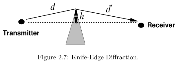
Diffraction is most commonly modeled by the Fresnel knife edge diffraction model due to its simplicity. The geometry of this model is shown in Figure 2.7, where the diffracting object is assumed to be asymptotically thin, which is not generally the case for hills, rough terrain, or wedge diffractors. In particular, this model does not consider diffractor parameters such as polarization, conductivity, and surfance roughness, which can lead to inaccuracies. The geometryof Figure 2.7 indicates that the diffracted signal travels distance $d+d^{\prime }$ resulting in a phase shift of $\varphi =2\pi (d+d^{\prime })/\lambda$. The geometry indicates that for $h$ small relative to $d$ and $d^{\prime }$, the singal must travel an additional distance relative to the LOS path of approximately $$△d=\frac{h^2}{2}\frac{d+d^{\prime }}{d{d}^{\prime }},$$ and the corresponding phase shift relative to the LOS path is approximately $$\varphi =\frac{2\pi △d}{\lambda }=\frac{\pi }{2}{v}^2,$$ where $$v=h\sqrt{\frac{2(d+d^{\prime })}{\lambda d{d}^{\prime }}}$$ is called the Fresnel-Kirchoff diffraction parameter. The path loss associated with knife-edge diffraction is generally a function of $v$.

Approximations for knife-edge diffraction path loss (in dB) relative to LOS path loss are given by Lee [14, Chapter 2] as

$$L(v)(dB)=\{\begin{array}{ll}20{\log }_{10}[0.5-0.62v]& -0.8\le v<0\\ 20{\log }_{10}\left[0.5e^{-.95v}\right]& 0\le v<1\\ 20{\log }_{10}\left[0.4-\sqrt{.1184-(.38-.1v{)}^2}\right]& 1\le v<2.4\\ 20{\log }_{10}[.225/v]& v>2.4\end{array}$$

A similar approximation can be found in [40]. The knife-edge diffraction model yields the following formula for the received diffracted signal: $$r(t)=\Re \left\{L(v)\sqrt{G_d}u(t-\tau )e^{\frac{-j\left(2\pi \left(d+d^{\prime }\right)\right)}{\lambda }}{e}^{j\left(2\pi f_{c}t+{\varphi }_0\right)},\right\}$$ where $\sqrt{G_d}$ is the antenna gain and $\tau =△d/c$ is the delay associated with the defracted ray relative to the LOS path.

In addition to the diffracted ray, there may also be multiple diffracted rays, or rays that are both reflected and diffracted. Models exist for including all possible permutations of reflection and diffraction [41]; however, the attenuation of the corresponding signal components is generally so large that these components are negligible relative to the noise.

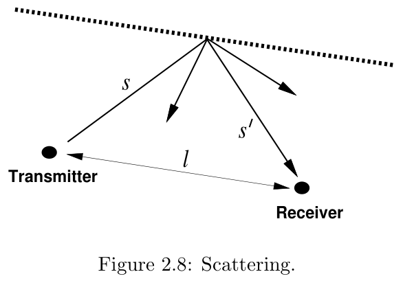
A scattered ray, shown in Figure 2.8 by the segments $s^{\prime }$ and $s$, has a path loss proportional to the product of $s$ and $s^{\prime }$. This multiplicative dependence is due to the additional spreading loss the ray experiences after scattering. The received signal due to a scattered ray is given by the bistatic radar equation [42]: $$r(t)=\Re \left\{u(t-\tau )\frac{\lambda \sqrt{G_s\sigma }{e}^{-j\left(2\pi \left(s+s^{\prime }\right)/\lambda \right)}}{(4\pi {)}^{3/2}s{s}^{\prime }}{e}^{j\left(2\pi f_{c}t+{\varphi }_0\right)}\right\},$$ where $\tau =(s+s^{\prime }-l)/c$ is the delay associated with the scattered ray, $\sigma$ (in $m^2$ ) is the radar cross section of the scattering object, which depends on the roughness, size, and shape of the scatterer, and $\sqrt{G_s}$ is the antenna gain.

In addition to the diffracted ray, there may also be multiple diffracted rays, or rays that are both reflected and diffracted. Models exist for including all possible permutations of reflection and diffraction [41]; however, the attenuation of the corresponding signal components is generally so large that these components are negligible relative to the noise.

A scattered ray, shown in Figure 2.8 by the segments $s^{\prime }$ and $s$, has a path loss proportional to the product of $s$ and $s^{\prime }$. This multiplicative dependence is due to the additional spreading loss the ray experiences after scattering. The received signal due to a scattered ray is given by the bistatic radar equation [42]: $$r(t)=\Re \left\{u(t-\tau )\frac{\lambda \sqrt{G_s\sigma }{e}^{-j\left(2\pi \left(s+s^{\prime }\right)/\lambda \right)}}{(4\pi {)}^{3/2}s{s}^{\prime }}{e}^{j\left(2\pi f_{c}t+{\varphi }_0\right)}\right\}$$ where $\tau =(s+s^{\prime }-l)/c$ is the delay associated with the scattered ray, $\sigma$ (in $m^2$ ) is the radar cross section of the scattering object, which depends on the roughness, size, and shape of the scatterer, and $G_s$ is the antenna gain.

The model assumes that the signal propagates from the transmitter to the scatterer based on free space propagation, and is then reradiated by the scatterer with transmit power equal to σ times the received power at the scatterer. From (2.25) the path loss associated with scattering is $$P_r(\mathrm{d}\mathrm{B}\mathrm{m})=P_t(\mathrm{d}\mathrm{B}\mathrm{m})+10{\log }_{10}\left(G_s\right)+10{\log }_{10}(\sigma )-30\log (4\pi )-20{\log }_{10}s-20{\log }_{10}\left(s^{\prime }\right).$$ Empirical values of $10\log 10\sigma$ were determined in [43] for different buildings in several cities. Results from this study indicate that $\sigma =10\log 10\sigma$ in $\text{db}{m}^2$ ranges from −4.5 $\text{db}{m}^2$ to 55.7 $\text{db}{m}^2$ , where $\text{db}{m}^2$ denotes the $\text{db}$ value of the $\sigma$ measurement with respect to one square meter.

The received signal is determined from the superposition of all the components due to the multiple rays. Thus, if we have a LOS ray, $N_r$ reflected rays, $N_d$ diffracted rays, and $N_s$ diffusely scattered rays, the total received signal is
$$\begin{array}{rl}{r}_{\text{total }}(t)& =\Re \{[\frac{\lambda }{4\pi }][\frac{\sqrt{G_l}u(t)e^{j(2\pi l)/\lambda }}{l}+\sum _{i=1}^{N_r}\frac{R_{x_i}\sqrt{G_{x_i}}u\left(t-{\tau }_i\right)e^{-j\left(2\pi r_i/\lambda \right)}}{r_i}\\ & +\sum _{j=1}^{N_d}{L}_j(v)\sqrt{G_{d_j}}u\left(t-{\tau }_j\right)e^{-j\left(2\pi \left(d_j+d_j^{\prime }\right)\right)/\lambda }{e}^{j\left(2\pi f_{c}t+{\varphi }_0\right)},\\ & +\sum _{k=1}^{N_s}\frac{{\sigma }_k\sqrt{G_{s_k}}u\left(t-{\tau }_k\right)e^{j\left(2\pi \left(s_k+s_k^{\prime }\right)\right)/\lambda }}{s_k{s}_k^{\prime }}]e^{j\left(2\pi f_{c}t+{\varphi }_0\right)}\},\end{array}$$ where ${\tau }_i$, ${\tau }_j$, ${\tau }_k$ is, respectively, the time delay of the given reflected, diffracted, or scattered ray normalized to the delay of the LOS ray, as defined above.

Any of these multipath components may have an additional attenuation factor if its propagation path is blocked by buildings or other objects.

---