手把手拆解：从零实现Llama3大模型（Python）（附代码）

自Meta 发布了开源大模型 llama3 系列，在多个关键基准测试中优于业界 SOTA 模型，并在代码生成任务上全面领先。太强了！10大开源大模型！

此后，开发者们便开始了本地部署和实现，比如 llama3 的中文实现、llama3 的纯 NumPy 实现等。

近期，有位名为「Nishant Aklecha」的开发者发布了一个从零开始实现 llama3 的存储库，包括跨多个头的注意力矩阵乘法、位置编码和每个层在内都有非常详细的解释。项目初期就已在 GitHub 上收获了 1.5k 的 star，足可见其含金量！

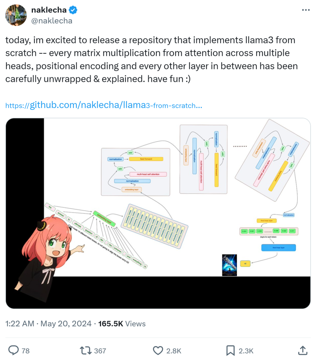
从零开始实现 llama3

接下来项目作者手把手教你如何从头开始实现 llama3。

项目地址：

https://github.com/naklecha/llama3-from-scratch

首先从 Meta 提供的 llama3 模型文件中加载张量。

下载地址：

https://llama.meta.com/llama-downloads/

接着是分词器（tokenizer），作者表示没打算自己实现分词器，因而借用了 Andrej Karpathy 的实现方式：

分词器的实现链接：

https://github.com/karpathy/minbpe

from pathlib import Path``import tiktoken``from tiktoken.load import load_tiktoken_bpe``import torch``import json``import matplotlib.pyplot as plt``tokenizer_path = "Meta-Llama-3-8B/tokenizer.model"``special_tokens = [`            `"<|begin_of_text|>",`            `"<|end_of_text|>",`            `"<|reserved_special_token_0|>",`            `"<|reserved_special_token_1|>",`            `"<|reserved_special_token_2|>",`            `"<|reserved_special_token_3|>",`            `"<|start_header_id|>",`            `"<|end_header_id|>",`            `"<|reserved_special_token_4|>",`            `"<|eot_id|>",  # end of turn`        `] + [f"<|reserved_special_token_{i}|>" for i in range (5, 256 - 5)] mergeable_ranks = load_tiktoken_bpe (tokenizer_path) tokenizer = tiktoken.Encoding (`    `name=Path (tokenizer_path).name,`    `pat_str=r"(?i:'s|'t|'re|'ve|'m|'ll|'d)|[^\r\n\p {L}\p {N}]?\p {L}+|\p {N}{1,3}| ?[^\s\p {L}\p {N}]+[\r\n]*|\s*[\r\n]+|\s+(?!\S)|\s+",`    `mergeable_ranks=mergeable_ranks,`    `special_tokens={token: len (mergeable_ranks) + i for i, token in enumerate (special_tokens)},``)``tokenizer.decode (tokenizer.encode ("hello world!"))

'hello world!'

上述步骤完成后，就是读取模型文件了。由于该研究是从头开始实现 llama3，因此代码一次只读取一个张量文件。

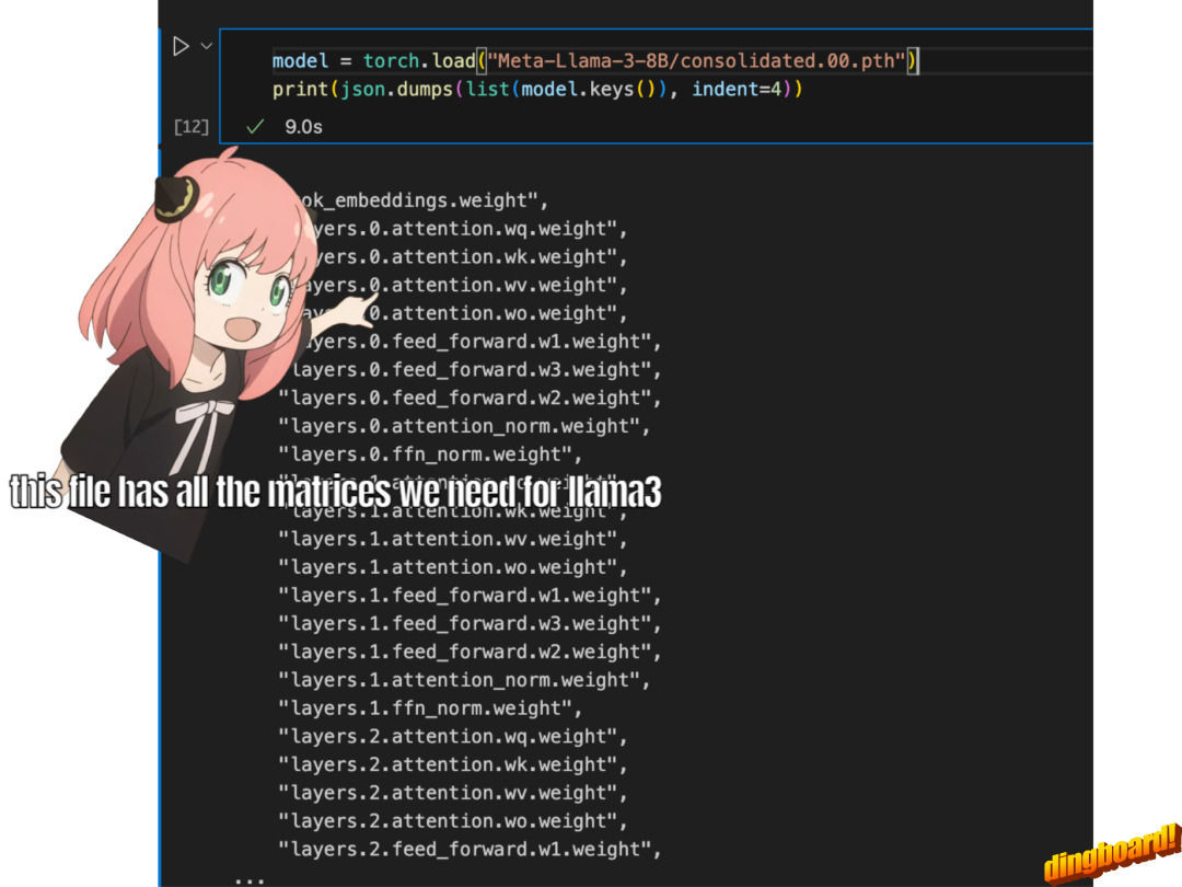
model = torch.load ("Meta-Llama-3-8B/consolidated.00.pth")``print (json.dumps (list (model.keys ())[:20], indent=4))

[`    `"tok_embeddings.weight",`    `"layers.0.attention.wq.weight",`    `"layers.0.attention.wk.weight",`    `"layers.0.attention.wv.weight",`    `"layers.0.attention.wo.weight",`    `"layers.0.feed_forward.w1.weight",`    `"layers.0.feed_forward.w3.weight",`    `"layers.0.feed_forward.w2.weight",`    `"layers.0.attention_norm.weight",`    `"layers.0.ffn_norm.weight",`    `"layers.1.attention.wq.weight",`    `"layers.1.attention.wk.weight",`    `"layers.1.attention.wv.weight",`    `"layers.1.attention.wo.weight",`    `"layers.1.feed_forward.w1.weight",`    `"layers.1.feed_forward.w3.weight",`    `"layers.1.feed_forward.w2.weight",`    `"layers.1.attention_norm.weight",`    `"layers.1.ffn_norm.weight",`    `"layers.2.attention.wq.weight"``]

with open ("Meta-Llama-3-8B/params.json", "r") as f:`    `config = json.load (f)``config

{'dim': 4096,` `'n_layers': 32,` `'n_heads': 32,` `'n_kv_heads': 8,` `'vocab_size': 128256,` `'multiple_of': 1024,` `'ffn_dim_multiplier': 1.3,` `'norm_eps': 1e-05,` `'rope_theta': 500000.0}

项目作者使用以下配置来推断模型细节：

• 模型有 32 个 transformer 层；

• 每个多头注意力块有 32 个头。

dim = config ["dim"]``n_layers = config ["n_layers"]``n_heads = config ["n_heads"]``n_kv_heads = config ["n_kv_heads"]``vocab_size = config ["vocab_size"]``multiple_of = config ["multiple_of"]``ffn_dim_multiplier = config ["ffn_dim_multiplier"]``norm_eps = config ["norm_eps"]``rope_theta = torch.tensor (config ["rope_theta"])

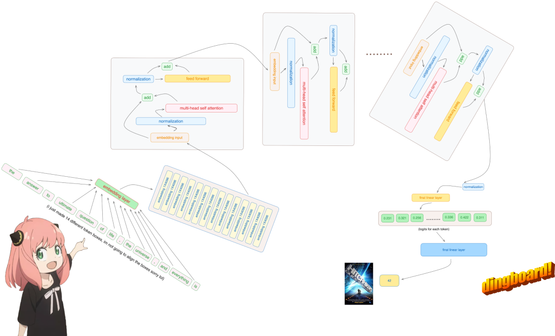
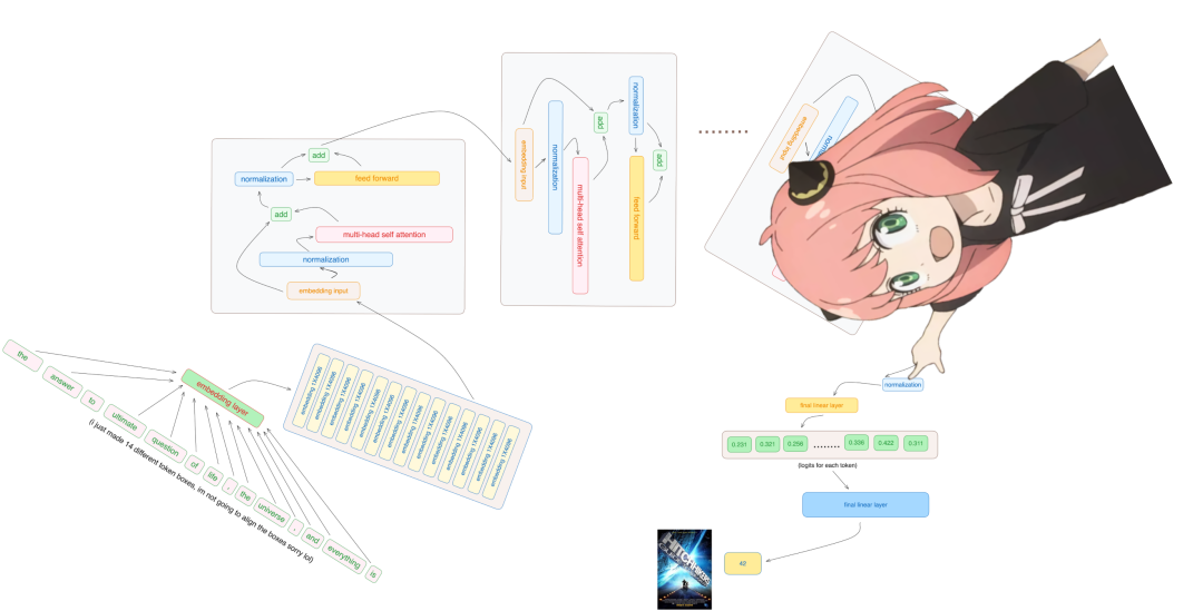
接下来的操作是将文本装换为 token，这里作者使用的是 tiktoken 库（一个用于 OpenAI 模型的 BPE tokeniser）。

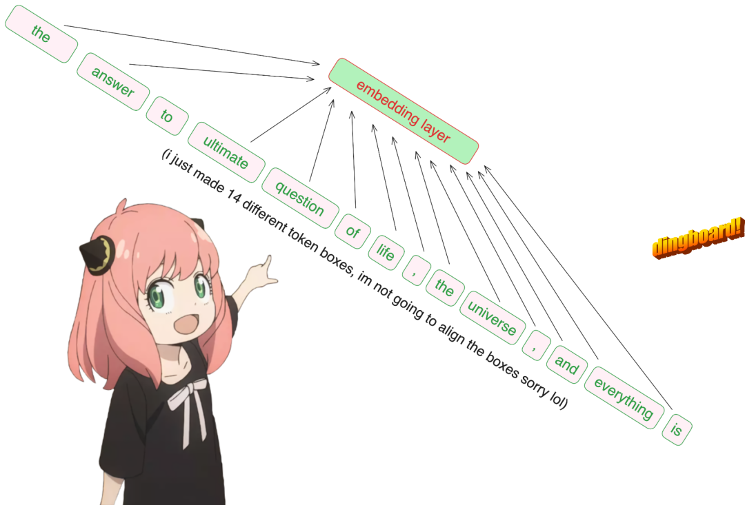
prompt = "the answer to the ultimate question of life, the universe, and everything is"``tokens = [128000] + tokenizer.encode (prompt)``print (tokens)``tokens = torch.tensor (tokens)``prompt_split_as_tokens = [tokenizer.decode ([token.item ()]) for token in tokens]``print (prompt_split_as_tokens)

[128000, 1820, 4320, 311, 279, 17139, 3488, 315, 2324, 11, 279, 15861, 11, 323, 4395, 374, 220]``['<|begin_of_text|>', 'the', ' answer', ' to', ' the', ' ultimate', ' question', ' of', ' life', ',', ' the', ' universe', ',', ' and', ' everything', ' is', ' ']

然后将 token 转换为嵌入。

embedding_layer = torch.nn.Embedding (vocab_size, dim)``embedding_layer.weight.data.copy_(model ["tok_embeddings.weight"])``token_embeddings_unnormalized = embedding_layer (tokens).to (torch.bfloat16)``token_embeddings_unnormalized.shape

torch.Size ([17, 4096])

将嵌入进行归一化。该研究使用均方根 RMS 算法进行归一化。不过，在这一步之后，张量形状不会改变，只是值进行了归一化。

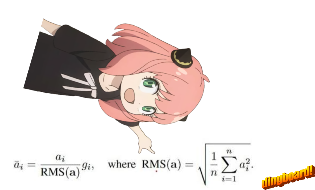
# def rms_norm (tensor, norm_weights):``#     rms = (tensor.pow (2).mean (-1, keepdim=True) + norm_eps)**0.5``#     return tensor * (norm_weights /rms)``def rms_norm (tensor, norm_weights):`    `return (tensor * torch.rsqrt (tensor.pow (2).mean (-1, keepdim=True) + norm_eps)) * norm_weights

构建 transformer 第一层。完成上述准备后，接着是构建 transformer 第一层：从模型文件中访问 layer.0（即第一层），归一化后嵌入维度仍然是 [17x4096] 。

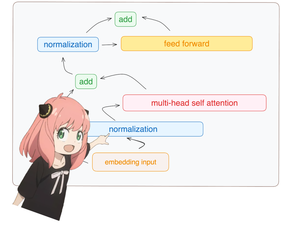
token_embeddings = rms_norm (token_embeddings_unnormalized, model ["layers.0.attention_norm.weight"])``token_embeddings.shape

torch.Size ([17, 4096])

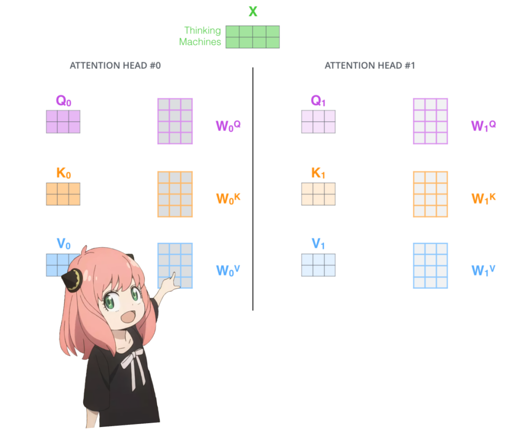
从头开始实现注意力。加载第一层 transformer 的注意力头：

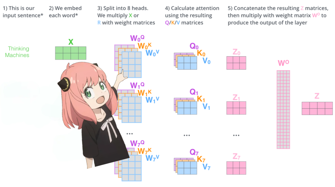
print (`    `model ["layers.0.attention.wq.weight"].shape,`    `model ["layers.0.attention.wk.weight"].shape,`    `model ["layers.0.attention.wv.weight"].shape,`    `model ["layers.0.attention.wo.weight"].shape``)``torch.Size ([4096, 4096]) torch.Size ([1024, 4096]) torch.Size ([1024, 4096]) torch.Size ([4096, 4096])

展开查询。展开来自多个注意力头的查询，得到的形状是 [32x128x4096]，这里，32 是 llama3 中注意力头的数量，128 是查询向量的大小，4096 是 token 嵌入的大小。

q_layer0 = model ["layers.0.attention.wq.weight"]``head_dim = q_layer0.shape [0] //n_heads``q_layer0 = q_layer0.view (n_heads, head_dim, dim)``q_layer0.shape

torch.Size ([32, 128, 4096])

从头实现第一层的第一个头。访问第一层的查询权重矩阵，大小是 [128x4096]。

q_layer0_head0 = q_layer0 [0]``q_layer0_head0.shape

torch.Size ([128, 4096])

将查询权重与 token 嵌入相乘，从而得到 token 的查询，在这里你可以看到结果大小是 [17x128]。

q_per_token = torch.matmul (token_embeddings, q_layer0_head0.T)``q_per_token.shape

torch.Size ([17, 128])

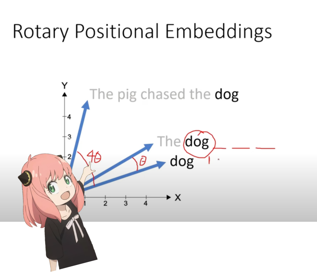
定位编码。现在处于这样一个阶段，即对提示符中的每个 token 都有一个查询向量，但是考虑单个查询向量，我们不知道其提示符中的位置。作者使用了 RoPE（旋转位置嵌入）来解决。

q_per_token_split_into_pairs = q_per_token.float ().view (q_per_token.shape [0], -1, 2)``q_per_token_split_into_pairs.shape

torch.Size ([17, 64, 2])

在上面的步骤中，该研究将查询向量分成对，并对每对应用旋转角度移位。

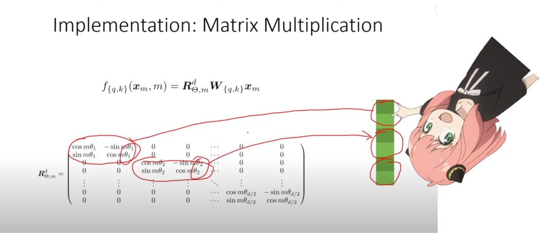
使用复数点积来旋转向量。

zero_to_one_split_into_64_parts = torch.tensor (range (64))/64``zero_to_one_split_into_64_parts

tensor ([0.0000, 0.0156, 0.0312, 0.0469, 0.0625, 0.0781, 0.0938, 0.1094, 0.1250,`        `0.1406, 0.1562, 0.1719, 0.1875, 0.2031, 0.2188, 0.2344, 0.2500, 0.2656,`        `0.2812, 0.2969, 0.3125, 0.3281, 0.3438, 0.3594, 0.3750, 0.3906, 0.4062,`        `0.4219, 0.4375, 0.4531, 0.4688, 0.4844, 0.5000, 0.5156, 0.5312, 0.5469,`        `0.5625, 0.5781, 0.5938, 0.6094, 0.6250, 0.6406, 0.6562, 0.6719, 0.6875,`        `0.7031, 0.7188, 0.7344, 0.7500, 0.7656, 0.7812, 0.7969, 0.8125, 0.8281,`        `0.8438, 0.8594, 0.8750, 0.8906, 0.9062, 0.9219, 0.9375, 0.9531, 0.9688,`        `0.9844])

freqs = 1.0 / (rope_theta ** zero_to_one_split_into_64_parts)``freqs

tensor ([1.0000e+00, 8.1462e-01, 6.6360e-01, 5.4058e-01, 4.4037e-01, 3.5873e-01,`        `2.9223e-01, 2.3805e-01, 1.9392e-01, 1.5797e-01, 1.2869e-01, 1.0483e-01,`        `8.5397e-02, 6.9566e-02, 5.6670e-02, 4.6164e-02, 3.7606e-02, 3.0635e-02,`        `2.4955e-02, 2.0329e-02, 1.6560e-02, 1.3490e-02, 1.0990e-02, 8.9523e-03,`        `7.2927e-03, 5.9407e-03, 4.8394e-03, 3.9423e-03, 3.2114e-03, 2.6161e-03,`        `2.1311e-03, 1.7360e-03, 1.4142e-03, 1.1520e-03, 9.3847e-04, 7.6450e-04,`        `6.2277e-04, 5.0732e-04, 4.1327e-04, 3.3666e-04, 2.7425e-04, 2.2341e-04,`        `1.8199e-04, 1.4825e-04, 1.2077e-04, 9.8381e-05, 8.0143e-05, 6.5286e-05,`        `5.3183e-05, 4.3324e-05, 3.5292e-05, 2.8750e-05, 2.3420e-05, 1.9078e-05,`        `1.5542e-05, 1.2660e-05, 1.0313e-05, 8.4015e-06, 6.8440e-06, 5.5752e-06,`        `4.5417e-06, 3.6997e-06, 3.0139e-06, 2.4551e-06])

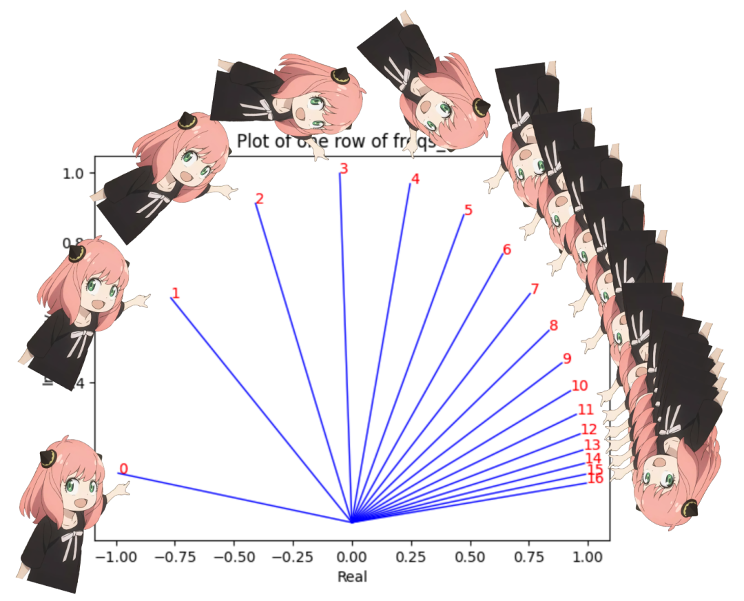
freqs_for_each_token = torch.outer (torch.arange (17), freqs)``freqs_cis = torch.polar (torch.ones_like (freqs_for_each_token), freqs_for_each_token)``freqs_cis.shape``# viewing tjhe third row of freqs_cis``value = freqs_cis [3]``plt.figure ()``for i, element in enumerate (value [:17]):`    `plt.plot ([0, element.real], [0, element.imag], color='blue', linewidth=1, label=f"Index: {i}")`    `plt.annotate (f"{i}", xy=(element.real, element.imag), color='red')`    `plt.xlabel ('Real')`    `plt.ylabel ('Imaginary')`    `plt.title ('Plot of one row of freqs_cis')`    `plt.show ()

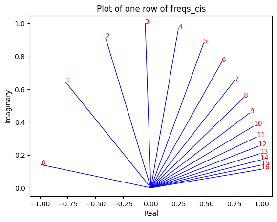
现在每个 token 查询都有了复数。

q_per_token_as_complex_numbers = torch.view_as_complex (q_per_token_split_into_pairs)``q_per_token_as_complex_numbers.shape

torch.Size ([17, 64])

q_per_token_as_complex_numbers_rotated = q_per_token_as_complex_numbers * freqs_cis``q_per_token_as_complex_numbers_rotated.shape

torch.Size ([17, 64])

旋转后的向量。

q_per_token_split_into_pairs_rotated = torch.view_as_real (q_per_token_as_complex_numbers_rotated)``q_per_token_split_into_pairs_rotated.shape

torch.Size ([17, 64, 2])

现在有了一个新的查询向量 (旋转查询向量)，形状为 [17x128]，其中 17 是 token 数量，128 是查询向量的维度。

q_per_token_rotated = q_per_token_split_into_pairs_rotated.view (q_per_token.shape)``q_per_token_rotated.shape

torch.Size ([17, 128])

键（几乎和查询一样），键也生成维度为 128 的键向量。键的权重只有查询的 1/4，这是因为键的权重在 4 个头之间共享，以减少所需的计算量，键也会被旋转以添加位置信息，就像查询一样。

k_layer0 = model ["layers.0.attention.wk.weight"]``k_layer0 = k_layer0.view (n_kv_heads, k_layer0.shape [0] //n_kv_heads, dim)``k_layer0.shape

torch.Size ([8, 128, 4096])

k_layer0_head0 = k_layer0 [0]``k_layer0_head0.shape

torch.Size ([128, 4096])

k_per_token = torch.matmul (token_embeddings, k_layer0_head0.T)``k_per_token.shape

torch.Size ([17, 128])

k_per_token_split_into_pairs = k_per_token.float ().view (k_per_token.shape [0], -1, 2)``k_per_token_split_into_pairs.shape

torch.Size ([17, 64, 2])

k_per_token_as_complex_numbers = torch.view_as_complex (k_per_token_split_into_pairs)``k_per_token_as_complex_numbers.shape

torch.Size ([17, 64])

k_per_token_split_into_pairs_rotated = torch.view_as_real (k_per_token_as_complex_numbers * freqs_cis)``k_per_token_split_into_pairs_rotated.shape

torch.Size ([17, 64, 2])

k_per_token_rotated = k_per_token_split_into_pairs_rotated.view (k_per_token.shape)``k_per_token_rotated.shape

torch.Size ([17, 128])

每个 token 查询和键的旋转值如下，每个查询和键现在的形状都是 [17x128]。

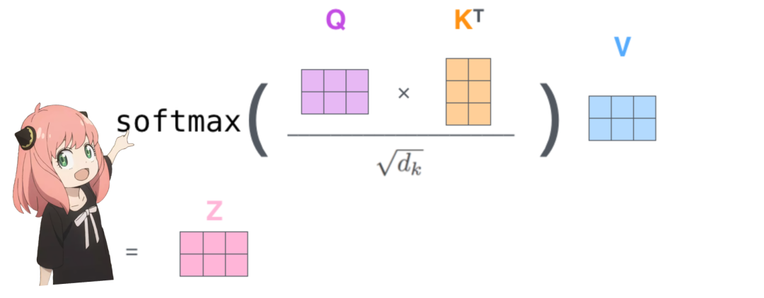
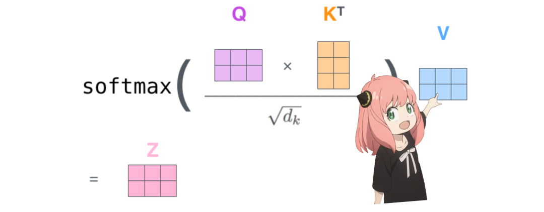
接下来一步是将查询和键矩阵相乘。注意力得分矩阵 (qk_per_token) 的形状为 [17x17]，其中 17 是提示中 token 的数量。

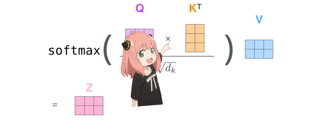
qk_per_token = torch.matmul (q_per_token_rotated, k_per_token_rotated.T)/(head_dim)**0.5``qk_per_token.shape

torch.Size ([17, 17])

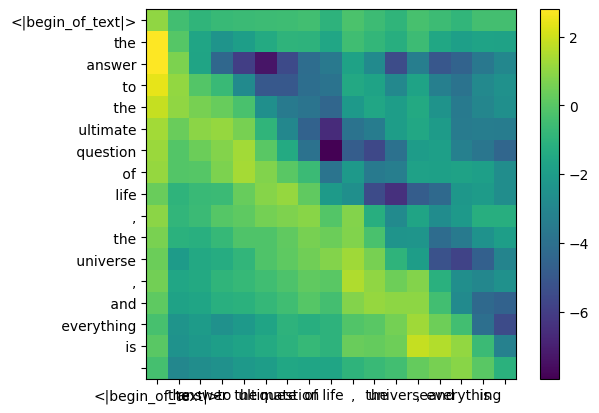
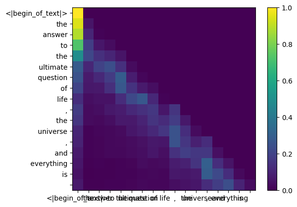
现在必须掩蔽查询键分数。

在 llama3 的训练过程中，未来 token 的 qk 分数被掩蔽。这是因为在训练期间，只学习使用过去的 token 来预测未来的 token。因此在推理过程中，将未来的 token 标记为零。

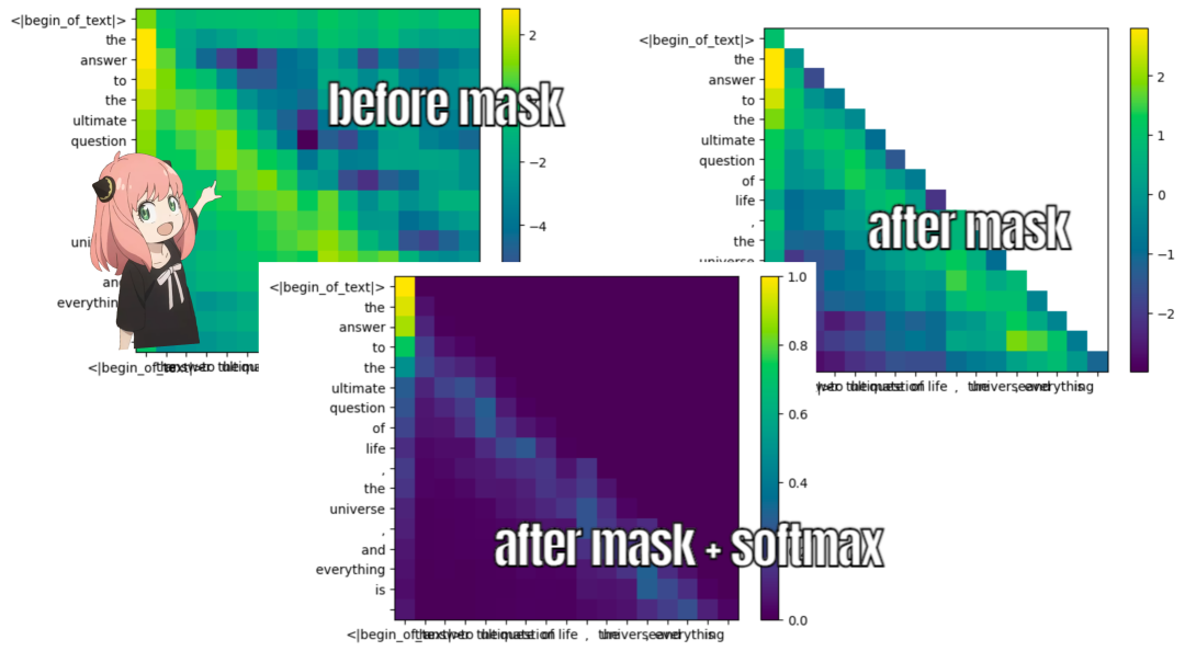
def display_qk_heatmap (qk_per_token):`    `_, ax = plt.subplots ()`    `im = ax.imshow (qk_per_token.to (float).detach (), cmap='viridis')`    `ax.set_xticks (range (len (prompt_split_as_tokens)))`    `ax.set_yticks (range (len (prompt_split_as_tokens)))`    `ax.set_xticklabels (prompt_split_as_tokens)`    `ax.set_yticklabels (prompt_split_as_tokens)`    `ax.figure.colorbar (im, ax=ax)`    `display_qk_heatmap (qk_per_token)

mask = torch.full ((len (tokens), len (tokens)), float ("-inf"), device=tokens.device) mask = torch.triu (mask, diagonal=1) mask

tensor ([[0., -inf, -inf, -inf, -inf, -inf, -inf, -inf, -inf, -inf, -inf, -inf, -inf, -inf, -inf, -inf, -inf],`        `[0., 0., -inf, -inf, -inf, -inf, -inf, -inf, -inf, -inf, -inf, -inf, -inf, -inf, -inf, -inf, -inf],`        `[0., 0., 0., -inf, -inf, -inf, -inf, -inf, -inf, -inf, -inf, -inf, -inf, -inf, -inf, -inf, -inf],`        `[0., 0., 0., 0., -inf, -inf, -inf, -inf, -inf, -inf, -inf, -inf, -inf, -inf, -inf, -inf, -inf],`        `[0., 0., 0., 0., 0., -inf, -inf, -inf, -inf, -inf, -inf, -inf, -inf, -inf, -inf, -inf, -inf],`        `[0., 0., 0., 0., 0., 0., -inf, -inf, -inf, -inf, -inf, -inf, -inf, -inf, -inf, -inf, -inf],`        `[0., 0., 0., 0., 0., 0., 0., -inf, -inf, -inf, -inf, -inf, -inf, -inf, -inf, -inf, -inf],`        `[0., 0., 0., 0., 0., 0., 0., 0., -inf, -inf, -inf, -inf, -inf, -inf, -inf, -inf, -inf],`        `[0., 0., 0., 0., 0., 0., 0., 0., 0., -inf, -inf, -inf, -inf, -inf, -inf, -inf, -inf],`        `[0., 0., 0., 0., 0., 0., 0., 0., 0., 0., -inf, -inf, -inf, -inf, -inf, -inf, -inf],`        `[0., 0., 0., 0., 0., 0., 0., 0., 0., 0., 0., -inf, -inf, -inf, -inf, -inf, -inf],`        `[0., 0., 0., 0., 0., 0., 0., 0., 0., 0., 0., 0., -inf, -inf, -inf, -inf, -inf],`        `[0., 0., 0., 0., 0., 0., 0., 0., 0., 0., 0., 0., 0., -inf, -inf, -inf, -inf],`        `[0., 0., 0., 0., 0., 0., 0., 0., 0., 0., 0., 0., 0., 0., -inf, -inf, -inf],`        `[0., 0., 0., 0., 0., 0., 0., 0., 0., 0., 0., 0., 0., 0., 0., -inf, -inf],`        `[0., 0., 0., 0., 0., 0., 0., 0., 0., 0., 0., 0., 0., 0., 0., 0., -inf],`        `[0., 0., 0., 0., 0., 0., 0., 0., 0., 0., 0., 0., 0., 0., 0., 0., 0.]])

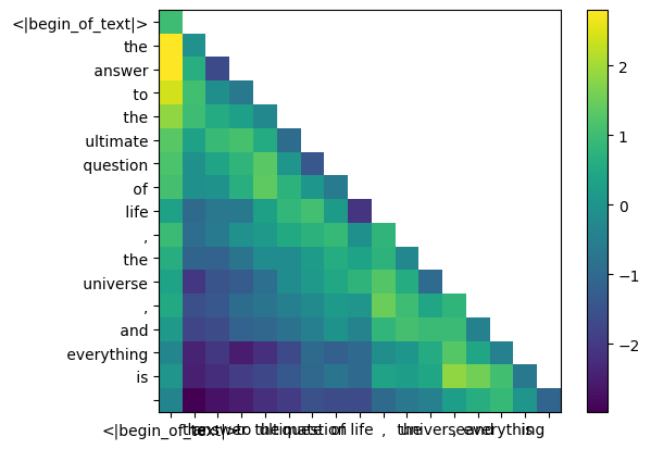
qk_per_token_after_masking = qk_per_token + mask``display_qk_heatmap (qk_per_token_after_masking)

qk_per_token_after_masking_after_softmax = torch.nn.functional.softmax (qk_per_token_after_masking, dim=1).to (torch.bfloat16) display_qk_heatmap (qk_per_token_after_masking_after_softmax)

值（几乎在注意力结束时）

这些分数 (0-1) 被用于确定每个 token 使用了多少值矩阵。

• 就像键一样，值权重也在 4 个注意力头之间共享（以节省计算量）

• 结果，下面的值权重矩阵形状为 [8x128x4096]

v_layer0 = model ["layers.0.attention.wv.weight"] v_layer0 = v_layer0.view (n_kv_heads, v_layer0.shape [0] //n_kv_heads, dim) v_layer0.shape

torch.Size ([8, 128, 4096])

第一层和第一个头的值权重矩阵如下所示。

v_layer0_head0 = v_layer0 [0] v_layer0_head0.shape

torch.Size ([128, 4096])

值向量如下图所示。

现在使用值权重来获取每个 token 的注意力值，其大小为 [17x128]，其中 17 为提示中的 token 数，128 为每个 token 的值向量维数。

v_per_token = torch.matmul (token_embeddings, v_layer0_head0.T)v_per_token.shape

torch.Size ([17, 128])

注意力如下图所示。

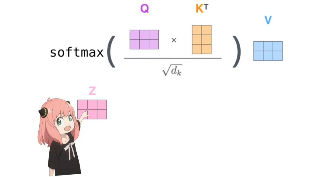
与每个 token 的值相乘后得到的注意力向量的形状为 [17*128]。

qkv_attention = torch.matmul (qk_per_token_after_masking_after_softmax, v_per_token) qkv_attention.shape

torch.Size ([17, 128])

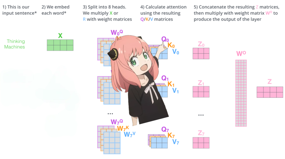
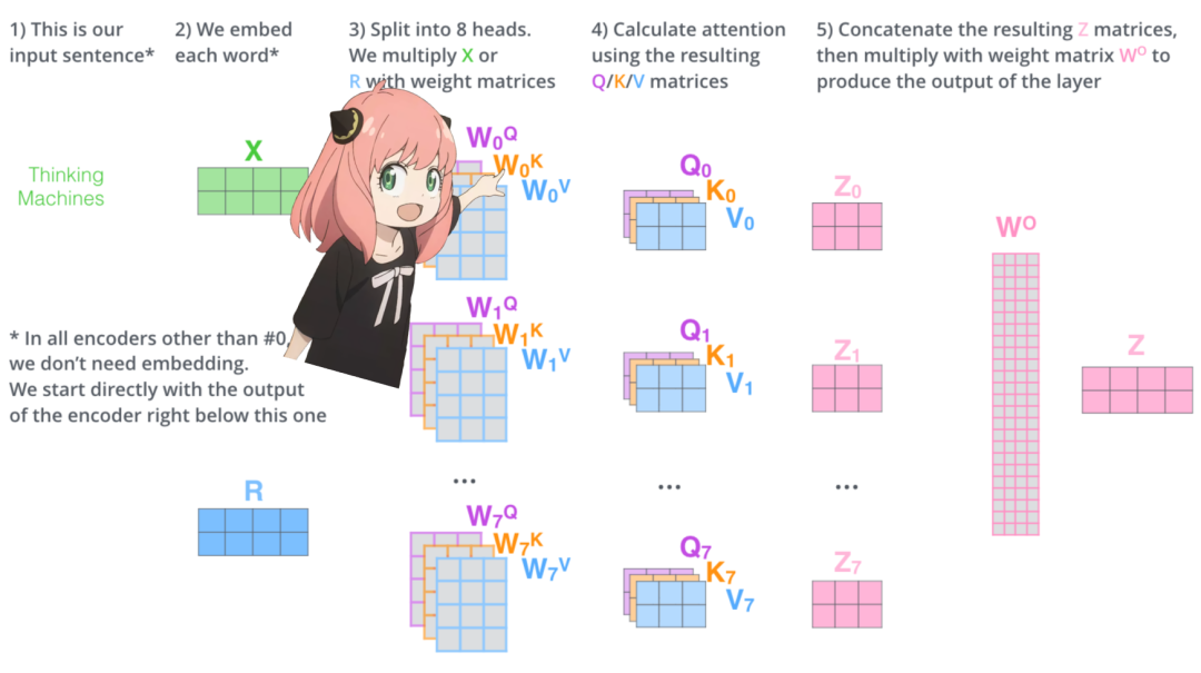
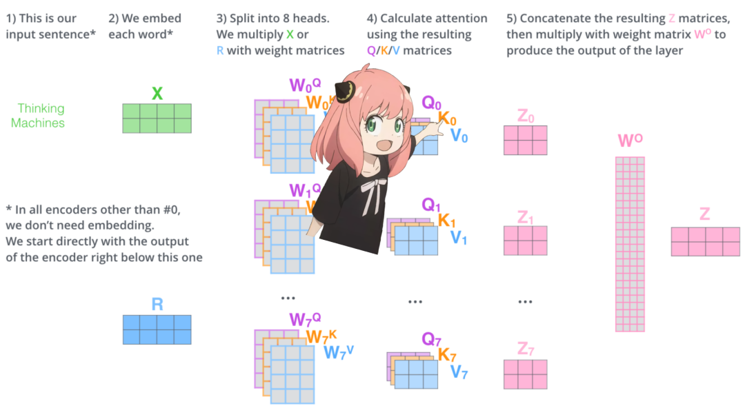
多头注意力与单头注意力如下图所示。

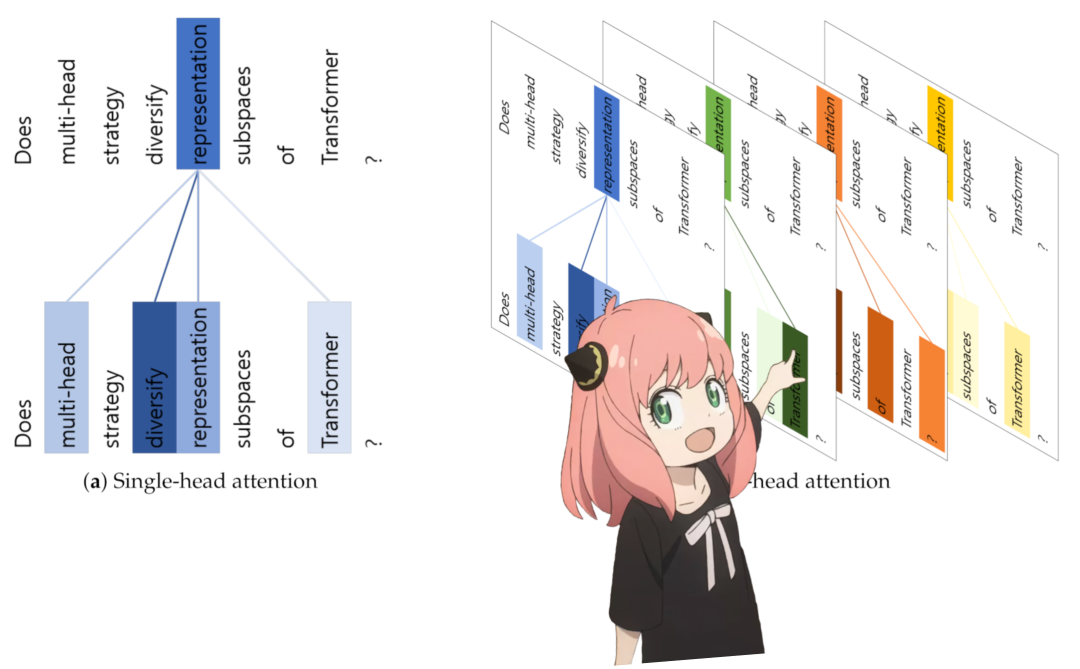
现在有了第一层和第一个头的注意力值。

接下来运行一个循环并执行与上面单元完全相同的数学运算，不过第一层中的每个头除外。

qkv_attention_store = []``for head in range (n_heads):`    `q_layer0_head = q_layer0 [head]`    `k_layer0_head = k_layer0 [head//4] # key weights are shared across 4 heads``v_layer0_head = v_layer0 [head//4] # value weights are shared across 4 heads``q_per_token = torch.matmul (token_embeddings, q_layer0_head.T)`    `k_per_token = torch.matmul (token_embeddings, k_layer0_head.T)`    `v_per_token = torch.matmul (token_embeddings, v_layer0_head.T)``   ``   `    `q_per_token_split_into_pairs = q_per_token.float ().view (q_per_token.shape [0], -1, 2)`    `q_per_token_as_complex_numbers = torch.view_as_complex (q_per_token_split_into_pairs)`    `q_per_token_split_into_pairs_rotated = torch.view_as_real (q_per_token_as_complex_numbers * freqs_cis [:len (tokens)])`    `q_per_token_rotated = q_per_token_split_into_pairs_rotated.view (q_per_token.shape)``   ``   `    `k_per_token_split_into_pairs = k_per_token.float ().view (k_per_token.shape [0], -1, 2)`    `k_per_token_as_complex_numbers = torch.view_as_complex (k_per_token_split_into_pairs)`    `k_per_token_split_into_pairs_rotated = torch.view_as_real (k_per_token_as_complex_numbers * freqs_cis [:len (tokens)])`    `k_per_token_rotated = k_per_token_split_into_pairs_rotated.view (k_per_token.shape)``   ``   `    `qk_per_token = torch.matmul (q_per_token_rotated, k_per_token_rotated.T)/(128)**0.5``mask = torch.full ((len (tokens), len (tokens)), float ("-inf"), device=tokens.device)`    `mask = torch.triu (mask, diagonal=1)`    `qk_per_token_after_masking = qk_per_token + mask``qk_per_token_after_masking_after_softmax = torch.nn.functional.softmax (qk_per_token_after_masking, dim=1).to (torch.bfloat16)`    `qkv_attention = torch.matmul (qk_per_token_after_masking_after_softmax, v_per_token)`    `qkv_attention = torch.matmul (qk_per_token_after_masking_after_softmax, v_per_token)`    `qkv_attention_store.append (qkv_attention)``len (qkv_attention_store)

32

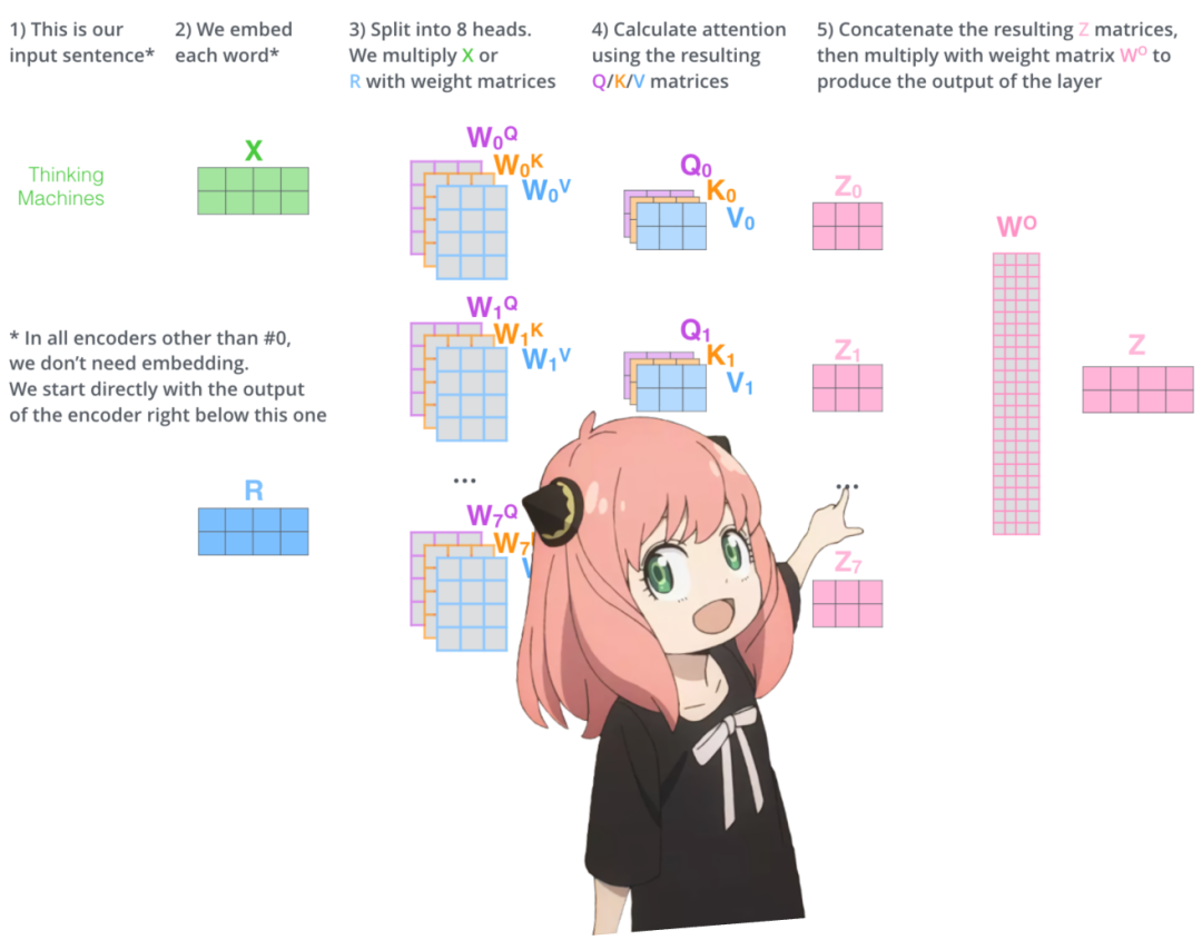
现在第一层上的所有 32 个头都有了 qkv_attention 矩阵，并在快结束的时候将所有注意力分数合并为一个大小为 [17x4096] 的大矩阵。

stacked_qkv_attention = torch.cat (qkv_attention_store, dim=-1) stacked_qkv_attention.shape

torch.Size ([17, 4096])

权重矩阵是最后的步骤之一。

第 0 层注意力要做的最后一件事是，对以下的权重矩阵进行乘法操作。

w_layer0 = model ["layers.0.attention.wo.weight"] w_layer0.shape

torch.Size ([4096, 4096])

这是一个简单的线性层，所以只做矩阵乘法（matmul）。

embedding_delta = torch.matmul (stacked_qkv_attention, w_layer0.T) embedding_delta.shape

torch.Size ([17, 4096])

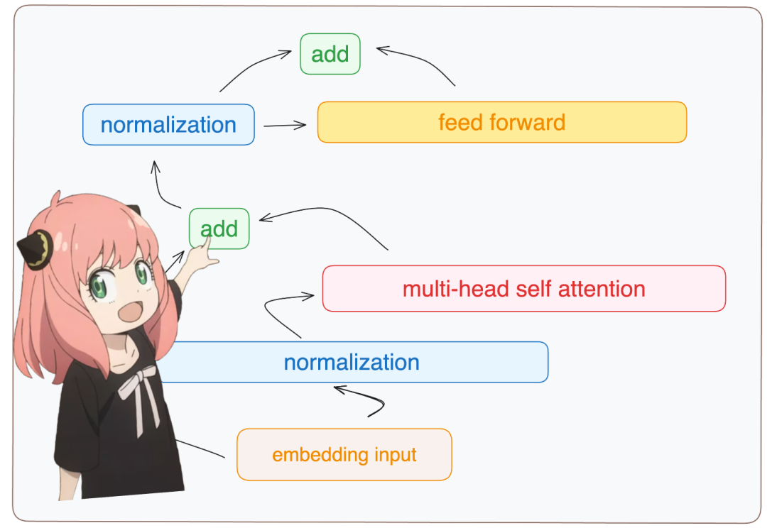
现在，注意力之后的嵌入值有了变化，并应该被添加到原始 token 嵌入中。

embedding_after_edit = token_embeddings_unnormalized + embedding_delta``embedding_after_edit.shape

torch.Size ([17, 4096])

归一化并在嵌入 delta 过程中运行一个前馈神经网络。

embedding_after_edit_normalized = rms_norm (embedding_after_edit, model ["layers.0.ffn_norm.weight"]) embedding_after_edit_normalized.shape

torch.Size ([17, 4096])

加载 ff 权重，并实现前馈网络。

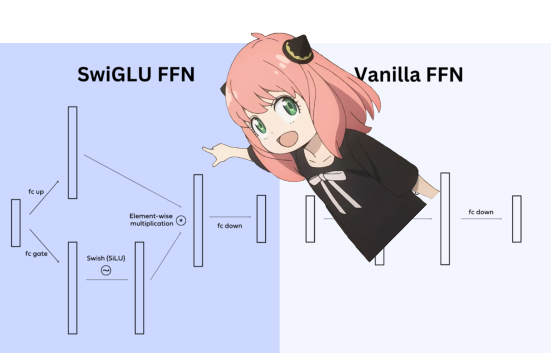
llama3 使用 SwiGLU前馈网络，该网络架构非常擅长在模型需要时添加非线性。当前，在 LLMs 中使用这一前馈网络是非常标准的做法。

w1 = model ["layers.0.feed_forward.w1.weight"] w2 = model ["layers.0.feed_forward.w2.weight"] w3 = model ["layers.0.feed_forward.w3.weight"] output_after_feedforward = torch.matmul (torch.functional.F.silu (torch.matmul (embedding_after_edit_normalized, w1.T)) * torch.matmul (embedding_after_edit_normalized, w3.T), w2.T) output_after_feedforward.shape

torch.Size ([17, 4096])

现在终于在第一层之后为每个 token 提供了新的编辑后的嵌入，并且在完成之前只剩下 31 层需要处理（one for loop away）。

你可以想象这个编辑后的嵌入拥有在第一层上所有查询的信息。现在每一层将在所问问题上编码越来越复杂的查询，直到得到的嵌入了解所需的下一个 token 的一切。

layer_0_embedding = embedding_after_edit+output_after_feedforward``layer_0_embedding.shape

torch.Size ([17, 4096])

之前为每一层做的所有事情，都可以一次性完成。

final_embedding = token_embeddings_unnormalized``for layer in range (n_layers):`    `qkv_attention_store = []`    `layer_embedding_norm = rms_norm (final_embedding, model [f"layers.{layer}.attention_norm.weight"])`    `q_layer = model [f"layers.{layer}.attention.wq.weight"]`    `q_layer = q_layer.view (n_heads, q_layer.shape [0] //n_heads, dim)`    `k_layer = model [f"layers.{layer}.attention.wk.weight"]`    `k_layer = k_layer.view (n_kv_heads, k_layer.shape [0] //n_kv_heads, dim)`    `v_layer = model [f"layers.{layer}.attention.wv.weight"]`    `v_layer = v_layer.view (n_kv_heads, v_layer.shape [0] //n_kv_heads, dim)`    `w_layer = model [f"layers.{layer}.attention.wo.weight"]`    `for head in range (n_heads):`        `q_layer_head = q_layer [head]`        `k_layer_head = k_layer [head//4]`        `v_layer_head = v_layer [head//4]`        `q_per_token = torch.matmul (layer_embedding_norm, q_layer_head.T)`        `k_per_token = torch.matmul (layer_embedding_norm, k_layer_head.T)`        `v_per_token = torch.matmul (layer_embedding_norm, v_layer_head.T)`        `q_per_token_split_into_pairs = q_per_token.float ().view (q_per_token.shape [0], -1, 2)`        `q_per_token_as_complex_numbers = torch.view_as_complex (q_per_token_split_into_pairs)`        `q_per_token_split_into_pairs_rotated = torch.view_as_real (q_per_token_as_complex_numbers * freqs_cis)`        `q_per_token_rotated = q_per_token_split_into_pairs_rotated.view (q_per_token.shape)`        `k_per_token_split_into_pairs = k_per_token.float ().view (k_per_token.shape [0], -1, 2)`        `k_per_token_as_complex_numbers = torch.view_as_complex (k_per_token_split_into_pairs)`        `k_per_token_split_into_pairs_rotated = torch.view_as_real (k_per_token_as_complex_numbers * freqs_cis)`        `k_per_token_rotated = k_per_token_split_into_pairs_rotated.view (k_per_token.shape)`        `qk_per_token = torch.matmul (q_per_token_rotated, k_per_token_rotated.T)/(128)**0.5`        `mask = torch.full ((len (token_embeddings_unnormalized), len (token_embeddings_unnormalized)), float ("-inf"))`        `mask = torch.triu (mask, diagonal=1)`        `qk_per_token_after_masking = qk_per_token + mask`        `qk_per_token_after_masking_after_softmax = torch.nn.functional.softmax (qk_per_token_after_masking, dim=1).to (torch.bfloat16)`        `qkv_attention = torch.matmul (qk_per_token_after_masking_after_softmax, v_per_token)`        `qkv_attention_store.append (qkv_attention)``   ``   `    `stacked_qkv_attention = torch.cat (qkv_attention_store, dim=-1)`    `w_layer = model [f"layers.{layer}.attention.wo.weight"]`    `embedding_delta = torch.matmul (stacked_qkv_attention, w_layer.T)`    `embedding_after_edit = final_embedding + embedding_delta`    `embedding_after_edit_normalized = rms_norm (embedding_after_edit, model [f"layers.{layer}.ffn_norm.weight"])`    `w1 = model [f"layers.{layer}.feed_forward.w1.weight"]`    `w2 = model [f"layers.{layer}.feed_forward.w2.weight"]`    `w3 = model [f"layers.{layer}.feed_forward.w3.weight"]`    `output_after_feedforward = torch.matmul (torch.functional.F.silu (torch.matmul (embedding_after_edit_normalized, w1.T)) * torch.matmul (embedding_after_edit_normalized, w3.T), w2.T)`    `final_embedding = embedding_after_edit+output_after_feedforward

现在有了最终的嵌入，即该模型对下一个 token 的最佳猜测。该嵌入的形状与常见的 token 嵌入 [17x4096] 相同，其中 17 为 token 数，4096 为嵌入维数。

final_embedding = rms_norm (final_embedding, model ["norm.weight"]) final_embedding.shape

torch.Size ([17, 4096])

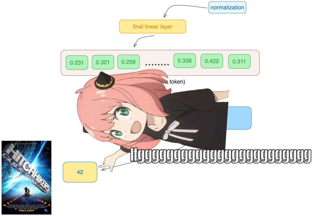
将该嵌入解码为 token 值。

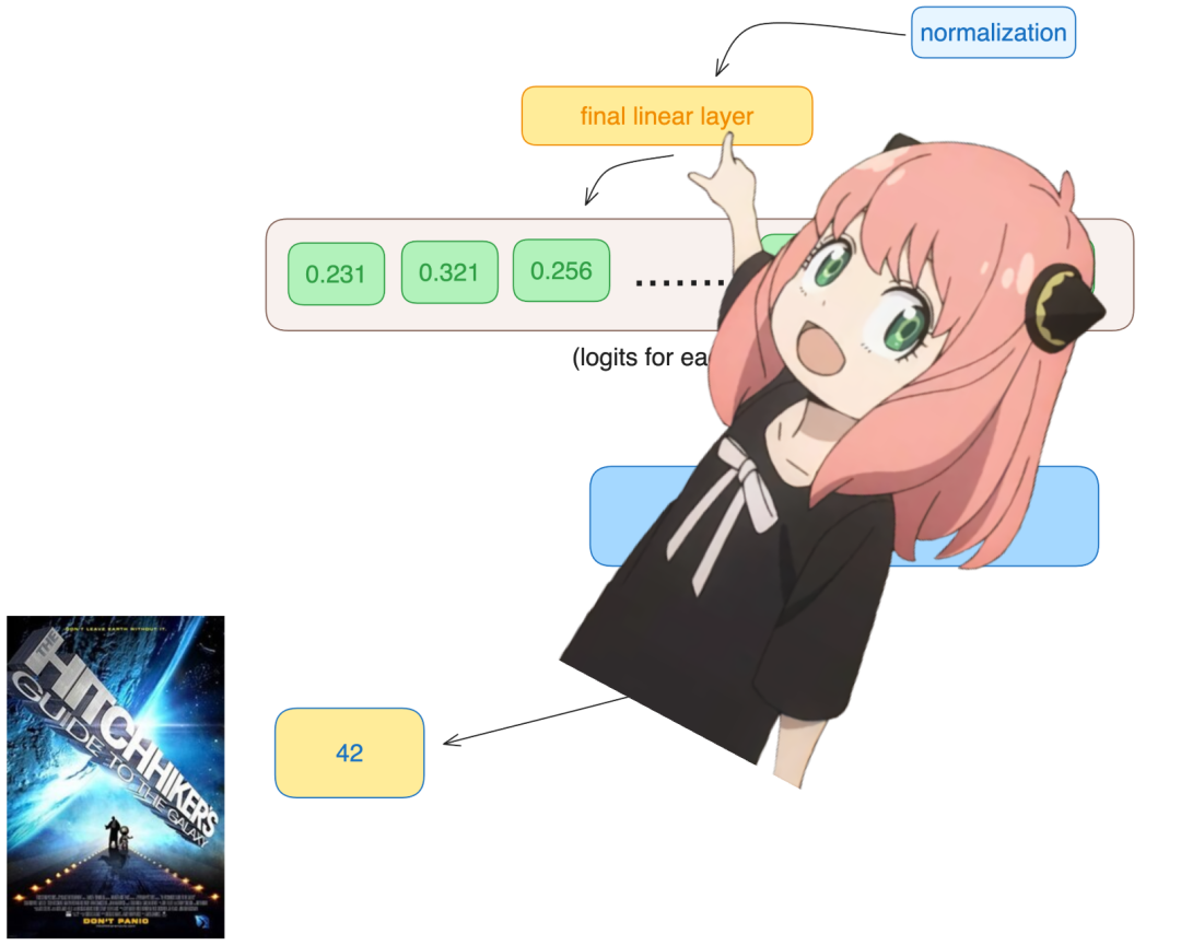
使用该输入解码器将最终的嵌入转换为一个 token。

model ["output.weight"].shape

torch.Size ([128256, 4096])

使用最后 token 的嵌入来预测下一个值。在示例中，42 是「生命、宇宙和万物终极问题的答案是什么」的答案，根据《银河系漫游指南》一书，大多数现代 LLMs 都会回答 42，应该验证了整个代码。

logits = torch.matmul (final_embedding [-1], model ["output.weight"].T) logits.shape

torch.Size ([128256])

模型预测 token 数 2983 为下一个 token，这是 42 的 token 数吗？以下是最后的代码单元。

next_token = torch.argmax (logits, dim=-1) next_token

tensor (2983)

最后，启动。

tokenizer.decode ([next_token.item ()])

'42'

如何学习大模型 AI ？

由于新岗位的生产效率，要优于被取代岗位的生产效率，所以实际上整个社会的生产效率是提升的。

但是具体到个人，只能说是：

“最先掌握AI的人，将会比较晚掌握AI的人有竞争优势”。

这句话，放在计算机、互联网、移动互联网的开局时期，都是一样的道理。

我在一线互联网企业工作十余年里，指导过不少同行后辈。帮助很多人得到了学习和成长。

我意识到有很多经验和知识值得分享给大家，也可以通过我们的能力和经验解答大家在人工智能学习中的很多困惑，所以在工作繁忙的情况下还是坚持各种整理和分享。但苦于知识传播途径有限，很多互联网行业朋友无法获得正确的资料得到学习提升，故此将并将重要的AI大模型资料包括AI大模型入门学习思维导图、精品AI大模型学习书籍手册、视频教程、实战学习等录播视频免费分享出来。

第一阶段（10天）：初阶应用

该阶段让大家对大模型 AI有一个最前沿的认识，对大模型 AI 的理解超过 95% 的人，可以在相关讨论时发表高级、不跟风、又接地气的见解，别人只会和 AI 聊天，而你能调教 AI，并能用代码将大模型和业务衔接。

• 大模型 AI 能干什么？
• 大模型是怎样获得「智能」的？
• 用好 AI 的核心心法
• 大模型应用业务架构
• 大模型应用技术架构
• 代码示例：向 GPT-3.5 灌入新知识
• 提示工程的意义和核心思想
• Prompt 典型构成
• 指令调优方法论
• 思维链和思维树
• Prompt 攻击和防范
• …

第二阶段（30天）：高阶应用

该阶段我们正式进入大模型 AI 进阶实战学习，学会构造私有知识库，扩展 AI 的能力。快速开发一个完整的基于 agent 对话机器人。掌握功能最强的大模型开发框架，抓住最新的技术进展，适合 Python 和 JavaScript 程序员。

• 为什么要做 RAG
• 搭建一个简单的 ChatPDF
• 检索的基础概念
• 什么是向量表示（Embeddings）
• 向量数据库与向量检索
• 基于向量检索的 RAG
• 搭建 RAG 系统的扩展知识
• 混合检索与 RAG-Fusion 简介
• 向量模型本地部署
• …

第三阶段（30天）：模型训练

恭喜你，如果学到这里，你基本可以找到一份大模型 AI相关的工作，自己也能训练 GPT 了！通过微调，训练自己的垂直大模型，能独立训练开源多模态大模型，掌握更多技术方案。

到此为止，大概2个月的时间。你已经成为了一名“AI小子”。那么你还想往下探索吗？

• 为什么要做 RAG
• 什么是模型
• 什么是模型训练
• 求解器 & 损失函数简介
• 小实验2：手写一个简单的神经网络并训练它
• 什么是训练/预训练/微调/轻量化微调
• Transformer结构简介
• 轻量化微调
• 实验数据集的构建
• …

第四阶段（20天）：商业闭环

对全球大模型从性能、吞吐量、成本等方面有一定的认知，可以在云端和本地等多种环境下部署大模型，找到适合自己的项目/创业方向，做一名被 AI 武装的产品经理。

• 硬件选型
• 带你了解全球大模型
• 使用国产大模型服务
• 搭建 OpenAI 代理
• 热身：基于阿里云 PAI 部署 Stable Diffusion
• 在本地计算机运行大模型
• 大模型的私有化部署
• 基于 vLLM 部署大模型
• 案例：如何优雅地在阿里云私有部署开源大模型
• 部署一套开源 LLM 项目
• 内容安全
• 互联网信息服务算法备案
• …

学习是一个过程，只要学习就会有挑战。天道酬勤，你越努力，就会成为越优秀的自己。

如果你能在15天内完成所有的任务，那你堪称天才。然而，如果你能完成 60-70% 的内容，你就已经开始具备成为一名大模型 AI 的正确特征了。

这份完整版的大模型 AI 学习资料已经上传CSDN，朋友们如果需要可以微信扫描下方CSDN官方认证二维码免费领取【保证100%免费】