


import numpy as np``import pandas as pd``import os, datetime``import tensorflow as tf``from tensorflow.keras.models import *``from tensorflow.keras.layers import *``print('Tensorflow version: {}'.format(tf.__version__))`` ``import matplotlib.pyplot as plt``plt.style.use('seaborn')`` ``import warnings``warnings.filterwarnings('ignore')`` ``physical_devices = tf.config.list_physical_devices()``print('Physical devices: {}'.format(physical_devices))`` ``# Filter out the CPUs and keep only the GPUs``gpus = [device for device in physical_devices if 'GPU' in device.device_type]`` ``# If GPUs are available, set memory growth to True``if len(gpus) > 0:` `tf.config.experimental.set_visible_devices(gpus[0], 'GPU')` `tf.config.experimental.set_memory_growth(gpus[0], True)` `print('GPU memory growth: True')
Tensorflow version: 2.9.1
Physical devices: [PhysicalDevice(name=‘/physical_device:CPU:0’, device_type=‘CPU’)]
Hyperparameters
batch_size = 32``seq_len = 128`` ``d_k = 256``d_v = 256``n_heads = 12``ff_dim = 256
Load IBM data
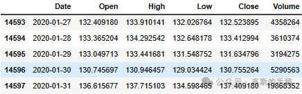
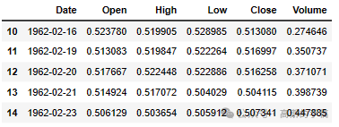
IBM_path = 'IBM.csv'`` ``df = pd.read_csv(IBM_path, delimiter=',', usecols=['Date', 'Open', 'High', 'Low', 'Close', 'Volume'])`` ``# Replace 0 to avoid dividing by 0 later on``df['Volume'].replace(to_replace=0, method='ffill', inplace=True)` `df.sort_values('Date', inplace=True)``df.tail()
df.head()
# print the shape of the dataset``print('Shape of the dataframe: {}'.format(df.shape))
Shape of the dataframe: (14588, 6)
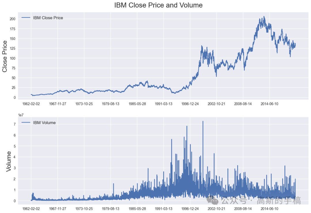
Plot daily IBM closing prices and volume
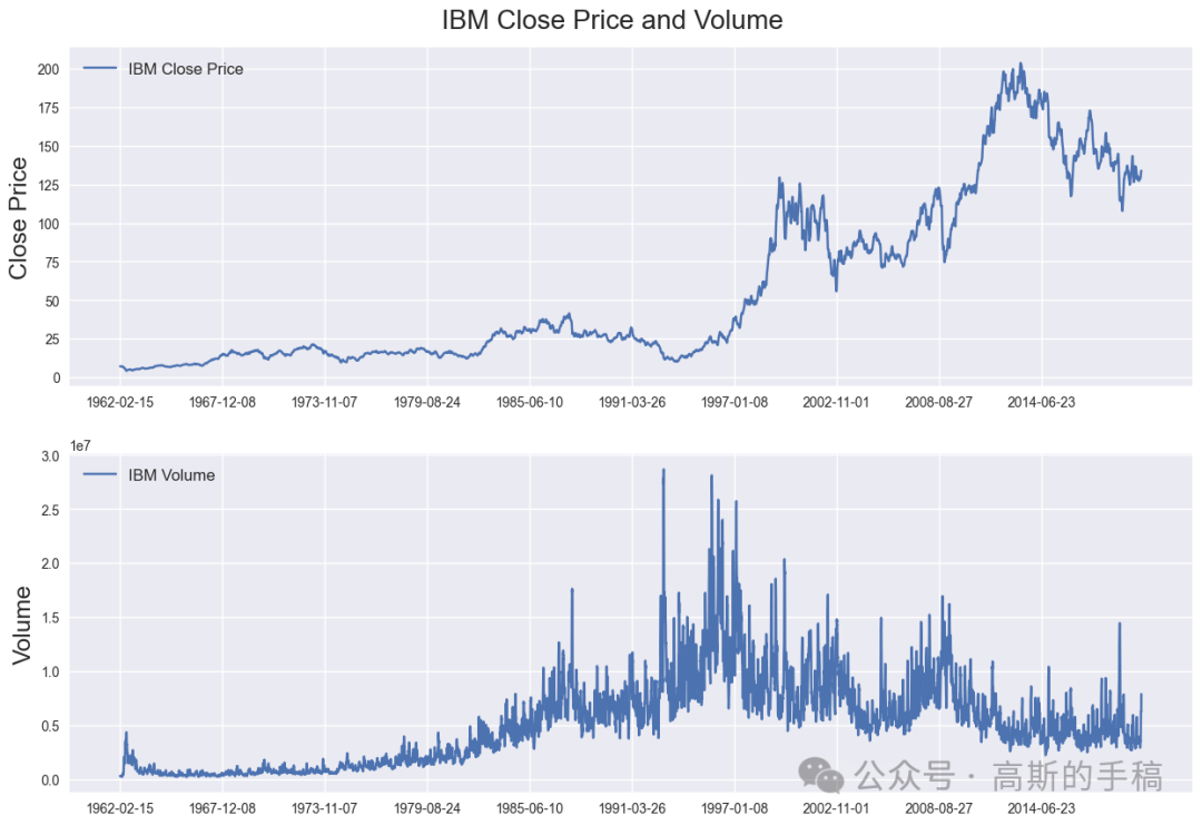
fig = plt.figure(figsize=(15,10))``st = fig.suptitle("IBM Close Price and Volume", fontsize=20)``st.set_y(0.92)`` ``ax1 = fig.add_subplot(211)``ax1.plot(df['Close'], label='IBM Close Price')``ax1.set_xticks(range(0, df.shape[0], 1464))``ax1.set_xticklabels(df['Date'].loc[::1464])``ax1.set_ylabel('Close Price', fontsize=18)``ax1.legend(loc="upper left", fontsize=12)`` ``ax2 = fig.add_subplot(212)``ax2.plot(df['Volume'], label='IBM Volume')``ax2.set_xticks(range(0, df.shape[0], 1464))``ax2.set_xticklabels(df['Date'].loc[::1464])``ax2.set_ylabel('Volume', fontsize=18)``ax2.legend(loc="upper left", fontsize=12)
Calculate normalized percentage change of all columns
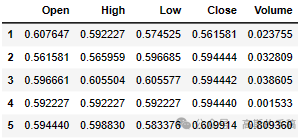
'''Calculate percentage change'''`` ``df['Open'] = df['Open'].pct_change() # Create arithmetic returns column``df['High'] = df['High'].pct_change() # Create arithmetic returns column``df['Low'] = df['Low'].pct_change() # Create arithmetic returns column``df['Close'] = df['Close'].pct_change() # Create arithmetic returns column``df['Volume'] = df['Volume'].pct_change()`` ``df.dropna(how='any', axis=0, inplace=True) # Drop all rows with NaN values`` ``###############################################################################``'''Create indexes to split dataset'''`` ``times = sorted(df.index.values)``last_10pct = sorted(df.index.values)[-int(0.1*len(times))] # Last 10% of series``last_20pct = sorted(df.index.values)[-int(0.2*len(times))] # Last 20% of series`` ``###############################################################################``'''Normalize price columns'''``#``min_return = min(df[(df.index < last_20pct)][['Open', 'High', 'Low', 'Close']].min(axis=0))``max_return = max(df[(df.index < last_20pct)][['Open', 'High', 'Low', 'Close']].max(axis=0))`` ``# Min-max normalize price columns (0-1 range)``df['Open'] = (df['Open'] - min_return) / (max_return - min_return)``df['High'] = (df['High'] - min_return) / (max_return - min_return)``df['Low'] = (df['Low'] - min_return) / (max_return - min_return)``df['Close'] = (df['Close'] - min_return) / (max_return - min_return)`` ``###############################################################################``'''Normalize volume column'''`` ``min_volume = df[(df.index < last_20pct)]['Volume'].min(axis=0)``max_volume = df[(df.index < last_20pct)]['Volume'].max(axis=0)`` ``# Min-max normalize volume columns (0-1 range)``df['Volume'] = (df['Volume'] - min_volume) / (max_volume - min_volume)`` ``###############################################################################``'''Create training, validation and test split'''`` ``df_train = df[(df.index < last_20pct)] # Training data are 80% of total data``df_val = df[(df.index >= last_20pct) & (df.index < last_10pct)]``df_test = df[(df.index >= last_10pct)]`` ``# Remove date column``df_train.drop(columns=['Date'], inplace=True)``df_val.drop(columns=['Date'], inplace=True)``df_test.drop(columns=['Date'], inplace=True)`` ``# Convert pandas columns into arrays``train_data = df_train.values``val_data = df_val.values``test_data = df_test.values``print('Training data shape: {}'.format(train_data.shape))``print('Validation data shape: {}'.format(val_data.shape))``print('Test data shape: {}'.format(test_data.shape))`` ``df_train.head()
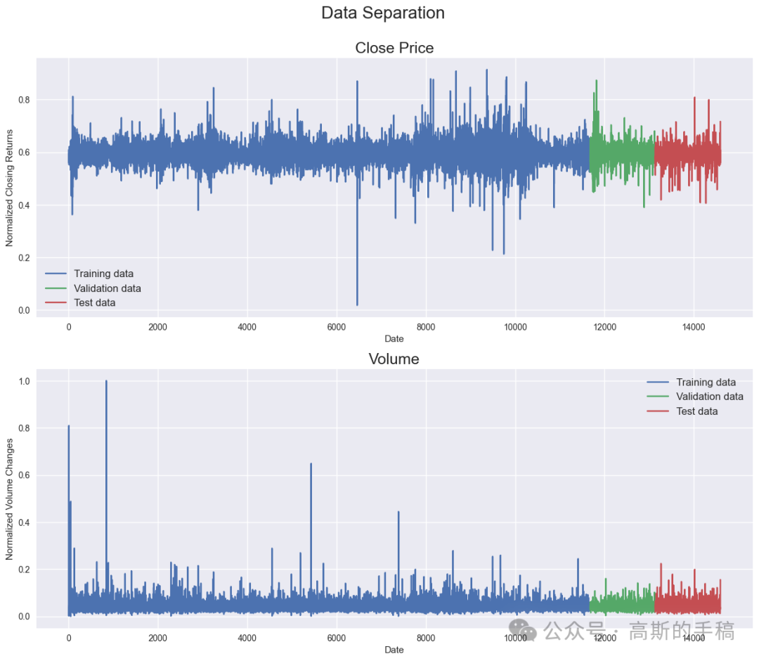
Training data shape: (11678, 5)
Validation data shape: (1460, 5)
Test data shape: (1459, 5)
Plot daily changes of close prices and volume
fig = plt.figure(figsize=(15,12))``st = fig.suptitle("Data Separation", fontsize=20)``st.set_y(0.95)`` ``###############################################################################`` ``ax1 = fig.add_subplot(211)``ax1.plot(np.arange(train_data.shape[0]), df_train['Close'], label='Training data')`` ``ax1.plot(np.arange(train_data.shape[0], `` train_data.shape[0]+val_data.shape[0]), df_val['Close'], label='Validation data')`` ``ax1.plot(np.arange(train_data.shape[0]+val_data.shape[0], `` train_data.shape[0]+val_data.shape[0]+test_data.shape[0]), df_test['Close'], label='Test data')``ax1.set_xlabel('Date')``ax1.set_ylabel('Normalized Closing Returns')``ax1.set_title("Close Price", fontsize=18)``ax1.legend(loc="best", fontsize=12)`` ``###############################################################################`` ``ax2 = fig.add_subplot(212)``ax2.plot(np.arange(train_data.shape[0]), df_train['Volume'], label='Training data')`` ``ax2.plot(np.arange(train_data.shape[0], `` train_data.shape[0]+val_data.shape[0]), df_val['Volume'], label='Validation data')`` ``ax2.plot(np.arange(train_data.shape[0]+val_data.shape[0], `` train_data.shape[0]+val_data.shape[0]+test_data.shape[0]), df_test['Volume'], label='Test data')``ax2.set_xlabel('Date')``ax2.set_ylabel('Normalized Volume Changes')``ax2.set_title("Volume", fontsize=18)``ax2.legend(loc="best", fontsize=12)
Create chunks of training, validation and test data
# Training data``X_train, y_train = [], []``for i in range(seq_len, len(train_data)):` `X_train.append(train_data[i-seq_len:i]) # Chunks of training data with a length of 128 df-rows` `y_train.append(train_data[:, 3][i]) #Value of 4th column (Close Price) of df-row 128+1``X_train, y_train = np.array(X_train), np.array(y_train)`` ``###############################################################################`` ``# Validation data``X_val, y_val = [], []``for i in range(seq_len, len(val_data)):` `X_val.append(val_data[i-seq_len:i])` `y_val.append(val_data[:, 3][i])``X_val, y_val = np.array(X_val), np.array(y_val)`` ``###############################################################################`` ``# Test data``X_test, y_test = [], []``for i in range(seq_len, len(test_data)):` `X_test.append(test_data[i-seq_len:i])` `y_test.append(test_data[:, 3][i])` `X_test, y_test = np.array(X_test), np.array(y_test)`` ``print('Training set shape', X_train.shape, y_train.shape)``print('Validation set shape', X_val.shape, y_val.shape)``print('Testing set shape' ,X_test.shape, y_test.shape)
Training set shape (11550, 128, 5) (11550,)
Validation set shape (1332, 128, 5) (1332,)
Testing set shape (1331, 128, 5) (1331,)
TimeVector
class Time2Vector(Layer):` `def __init__(self, seq_len, **kwargs):` `super(Time2Vector, self).__init__()` `self.seq_len = seq_len`` ` `def build(self, input_shape):` `'''Initialize weights and biases with shape (batch, seq_len)'''` `self.weights_linear = self.add_weight(name='weight_linear',` `shape=(int(self.seq_len),),` `initializer='uniform',` `trainable=True)` ` self.bias_linear = self.add_weight(name='bias_linear',` `shape=(int(self.seq_len),),` `initializer='uniform',` `trainable=True)` ` self.weights_periodic = self.add_weight(name='weight_periodic',` `shape=(int(self.seq_len),),` `initializer='uniform',` `trainable=True)`` ` `self.bias_periodic = self.add_weight(name='bias_periodic',` `shape=(int(self.seq_len),),` `initializer='uniform',` `trainable=True)`` ` `def call(self, x):` `'''Calculate linear and periodic time features'''` `x = tf.math.reduce_mean(x[:,:,:4], axis=-1)`` time_linear = self.weights_linear * x + self.bias_linear # Linear time feature` `time_linear = tf.expand_dims(time_linear, axis=-1) # Add dimension (batch, seq_len, 1)` ` time_periodic = tf.math.sin(tf.multiply(x, self.weights_periodic) + self.bias_periodic)` `time_periodic = tf.expand_dims(time_periodic, axis=-1) # Add dimension (batch, seq_len, 1)` `return tf.concat([time_linear, time_periodic], axis=-1) # shape = (batch, seq_len, 2)` ` def get_config(self): # Needed for saving and loading model with custom layer` `config = super().get_config().copy()` `config.update({'seq_len': self.seq_len})` `return config
Transformer
class SingleAttention(Layer):` `def __init__(self, d_k, d_v):` `super(SingleAttention, self).__init__()` `self.d_k = d_k` `self.d_v = d_v`` ` `def build(self, input_shape):` `self.query = Dense(self.d_k,`` input_shape=input_shape, `` kernel_initializer='glorot_uniform', `` bias_initializer='glorot_uniform')` ` self.key = Dense(self.d_k, `` input_shape=input_shape, `` kernel_initializer='glorot_uniform', `` bias_initializer='glorot_uniform')` ` self.value = Dense(self.d_v, `` input_shape=input_shape, `` kernel_initializer='glorot_uniform', `` bias_initializer='glorot_uniform')`` ` `def call(self, inputs): # inputs = (in_seq, in_seq, in_seq)` `q = self.query(inputs[0])` `k = self.key(inputs[1])`` ` `attn_weights = tf.matmul(q, k, transpose_b=True)` `attn_weights = tf.map_fn(lambda x: x/np.sqrt(self.d_k), attn_weights)` `attn_weights = tf.nn.softmax(attn_weights, axis=-1)` ` v = self.value(inputs[2])` `attn_out = tf.matmul(attn_weights, v)` `return attn_out` ` ``#############################################################################`` ``class MultiAttention(Layer):` `def __init__(self, d_k, d_v, n_heads):` `super(MultiAttention, self).__init__()` `self.d_k = d_k` `self.d_v = d_v` `self.n_heads = n_heads` `self.attn_heads = list()`` ` `def build(self, input_shape):` `for n in range(self.n_heads):` `self.attn_heads.append(SingleAttention(self.d_k, self.d_v))`` # input_shape[0]=(batch, seq_len, 7), input_shape[0][-1]=7 `` self.linear = Dense(input_shape[0][-1], `` input_shape=input_shape, `` kernel_initializer='glorot_uniform', `` bias_initializer='glorot_uniform')`` ` `def call(self, inputs):` `attn = [self.attn_heads[i](inputs) for i in range(self.n_heads)]` `concat_attn = tf.concat(attn, axis=-1)` `multi_linear = self.linear(concat_attn)` `return multi_linear` ` ``#############################################################################`` ``class TransformerEncoder(Layer):` `def __init__(self, d_k, d_v, n_heads, ff_dim, dropout=0.1, **kwargs):` `super(TransformerEncoder, self).__init__()` `self.d_k = d_k` `self.d_v = d_v` `self.n_heads = n_heads` `self.ff_dim = ff_dim` `self.attn_heads = list()` `self.dropout_rate = dropout`` ` `def build(self, input_shape):` `self.attn_multi = MultiAttention(self.d_k, self.d_v, self.n_heads)` `self.attn_dropout = Dropout(self.dropout_rate)` `self.attn_normalize = LayerNormalization(input_shape=input_shape, epsilon=1e-6)`` ` `self.ff_conv1D_1 = Conv1D(filters=self.ff_dim, kernel_size=1, activation='relu')` `# input_shape[0]=(batch, seq_len, 7), input_shape[0][-1] = 7`` self.ff_conv1D_2 = Conv1D(filters=input_shape[0][-1], kernel_size=1) `` self.ff_dropout = Dropout(self.dropout_rate)` `self.ff_normalize = LayerNormalization(input_shape=input_shape, epsilon=1e-6)`` def call(self, inputs): # inputs = (in_seq, in_seq, in_seq)` `attn_layer = self.attn_multi(inputs)` `attn_layer = self.attn_dropout(attn_layer)` `attn_layer = self.attn_normalize(inputs[0] + attn_layer)`` ` `ff_layer = self.ff_conv1D_1(attn_layer)` `ff_layer = self.ff_conv1D_2(ff_layer)` `ff_layer = self.ff_dropout(ff_layer)` `ff_layer = self.ff_normalize(inputs[0] + ff_layer)` `return ff_layer` ` ` `def get_config(self): # Needed for saving and loading model with custom layer` `config = super().get_config().copy()` `config.update({'d_k': self.d_k,` `'d_v': self.d_v,` `'n_heads': self.n_heads,` `'ff_dim': self.ff_dim,` `'attn_heads': self.attn_heads,` `'dropout_rate': self.dropout_rate})` `return config
Model
def create_model():` `'''Initialize time and transformer layers'''` `time_embedding = Time2Vector(seq_len)` `attn_layer1 = TransformerEncoder(d_k, d_v, n_heads, ff_dim)` `attn_layer2 = TransformerEncoder(d_k, d_v, n_heads, ff_dim)` `attn_layer3 = TransformerEncoder(d_k, d_v, n_heads, ff_dim)`` ` `'''Construct model'''` `in_seq = Input(shape=(seq_len, 5))` `x = time_embedding(in_seq)` `x = Concatenate(axis=-1)([in_seq, x])` `x = attn_layer1((x, x, x))` `x = attn_layer2((x, x, x))` `x = attn_layer3((x, x, x))` `x = GlobalAveragePooling1D(data_format='channels_first')(x)` `x = Dropout(0.1)(x)` `x = Dense(64, activation='relu')(x)` `x = Dropout(0.1)(x)` `out = Dense(1, activation='linear')(x)`` ` `model = Model(inputs=in_seq, outputs=out)` `model.compile(loss='mse', optimizer='adam', metrics=['mae', 'mape'])` `return model`` `` ``model = create_model()``model.summary()`` ``callback = tf.keras.callbacks.ModelCheckpoint('Transformer+TimeEmbedding.hdf5', `` monitor='val_loss', `` save_best_only=True, verbose=1)`` ``history = model.fit(X_train, y_train, `` batch_size=batch_size, `` epochs=35, `` callbacks=[callback],` `validation_data=(X_val, y_val))` ` ``model = tf.keras.models.load_model('Transformer+TimeEmbedding.hdf5',` `custom_objects={'Time2Vector': Time2Vector,`` 'SingleAttention': SingleAttention,` `'MultiAttention': MultiAttention,` `'TransformerEncoder': TransformerEncoder})`` `` ``###############################################################################``'''Calculate predictions and metrics'''`` ``#Calculate predication for training, validation and test data``train_pred = model.predict(X_train)``val_pred = model.predict(X_val)``test_pred = model.predict(X_test)`` ``#Print evaluation metrics for all datasets``train_eval = model.evaluate(X_train, y_train, verbose=0)``val_eval = model.evaluate(X_val, y_val, verbose=0)``test_eval = model.evaluate(X_test, y_test, verbose=0)``print(' ')``print('Evaluation metrics')``print('Training Data - Loss: {:.4f}, MAE: {:.4f}, MAPE: {:.4f}'.format(train_eval[0], train_eval[1], train_eval[2]))``print('Validation Data - Loss: {:.4f}, MAE: {:.4f}, MAPE: {:.4f}'.format(val_eval[0], val_eval[1], val_eval[2]))``print('Test Data - Loss: {:.4f}, MAE: {:.4f}, MAPE: {:.4f}'.format(test_eval[0], test_eval[1], test_eval[2]))`` ``###############################################################################``'''Display results'''`` ``fig = plt.figure(figsize=(15,20))``st = fig.suptitle("Transformer + TimeEmbedding Model", fontsize=22)``st.set_y(0.92)`` ``#Plot training data results``ax11 = fig.add_subplot(311)``ax11.plot(train_data[:, 3], label='IBM Closing Returns')``ax11.plot(np.arange(seq_len, train_pred.shape[0]+seq_len), train_pred, linewidth=3, label='Predicted IBM Closing Returns')``ax11.set_title("Training Data", fontsize=18)``ax11.set_xlabel('Date')``ax11.set_ylabel('IBM Closing Returns')``ax11.legend(loc="best", fontsize=12)`` ``#Plot validation data results``ax21 = fig.add_subplot(312)``ax21.plot(val_data[:, 3], label='IBM Closing Returns')``ax21.plot(np.arange(seq_len, val_pred.shape[0]+seq_len), val_pred, linewidth=3, label='Predicted IBM Closing Returns')``ax21.set_title("Validation Data", fontsize=18)``ax21.set_xlabel('Date')``ax21.set_ylabel('IBM Closing Returns')``ax21.legend(loc="best", fontsize=12)`` ``#Plot test data results``ax31 = fig.add_subplot(313)``ax31.plot(test_data[:, 3], label='IBM Closing Returns')``ax31.plot(np.arange(seq_len, test_pred.shape[0]+seq_len), test_pred, linewidth=3, label='Predicted IBM Closing Returns')``ax31.set_title("Test Data", fontsize=18)``ax31.set_xlabel('Date')``ax31.set_ylabel('IBM Closing Returns')``ax31.legend(loc="best", fontsize=12)
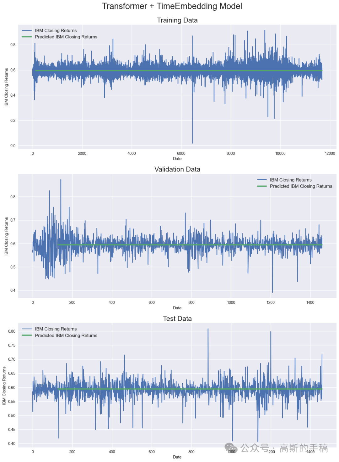
###############################################################################``'''Calculate predictions and metrics'''`` ``#Calculate predication for training, validation and test data``train_pred = model.predict(X_train)``val_pred = model.predict(X_val)``test_pred = model.predict(X_test)`` ``#Print evaluation metrics for all datasets``train_eval = model.evaluate(X_train, y_train, verbose=0)``val_eval = model.evaluate(X_val, y_val, verbose=0)``test_eval = model.evaluate(X_test, y_test, verbose=0)``print(' ')``print('Evaluation metrics')``print('Training Data - Loss: {:.4f}, MAE: {:.4f}, MAPE: {:.4f}'.format(train_eval[0], train_eval[1], train_eval[2]))``print('Validation Data - Loss: {:.4f}, MAE: {:.4f}, MAPE: {:.4f}'.format(val_eval[0], val_eval[1], val_eval[2]))``print('Test Data - Loss: {:.4f}, MAE: {:.4f}, MAPE: {:.4f}'.format(test_eval[0], test_eval[1], test_eval[2]))`` ``###############################################################################``'''Display results'''`` ``fig = plt.figure(figsize=(15,20))``st = fig.suptitle("Transformer + TimeEmbedding Model", fontsize=22)``st.set_y(0.92)`` ``#Plot training data results``ax11 = fig.add_subplot(311)``ax11.plot(train_data[:, 3], label='IBM Closing Returns')``ax11.plot(np.arange(seq_len, train_pred.shape[0]+seq_len), train_pred, linewidth=3, label='Predicted IBM Closing Returns')``ax11.set_title("Training Data", fontsize=18)``ax11.set_xlabel('Date')``ax11.set_ylabel('IBM Closing Returns')``ax11.legend(loc="best", fontsize=12)`` ``#Plot validation data results``ax21 = fig.add_subplot(312)``ax21.plot(val_data[:, 3], label='IBM Closing Returns')``ax21.plot(np.arange(seq_len, val_pred.shape[0]+seq_len), val_pred, linewidth=3, label='Predicted IBM Closing Returns')``ax21.set_title("Validation Data", fontsize=18)``ax21.set_xlabel('Date')``ax21.set_ylabel('IBM Closing Returns')``ax21.legend(loc="best", fontsize=12)`` ``#Plot test data results``ax31 = fig.add_subplot(313)``ax31.plot(test_data[:, 3], label='IBM Closing Returns')``ax31.plot(np.arange(seq_len, test_pred.shape[0]+seq_len), test_pred, linewidth=3, label='Predicted IBM Closing Returns')``ax31.set_title("Test Data", fontsize=18)``ax31.set_xlabel('Date')``ax31.set_ylabel('IBM Closing Returns')``ax31.legend(loc="best", fontsize=12)
Model metrics
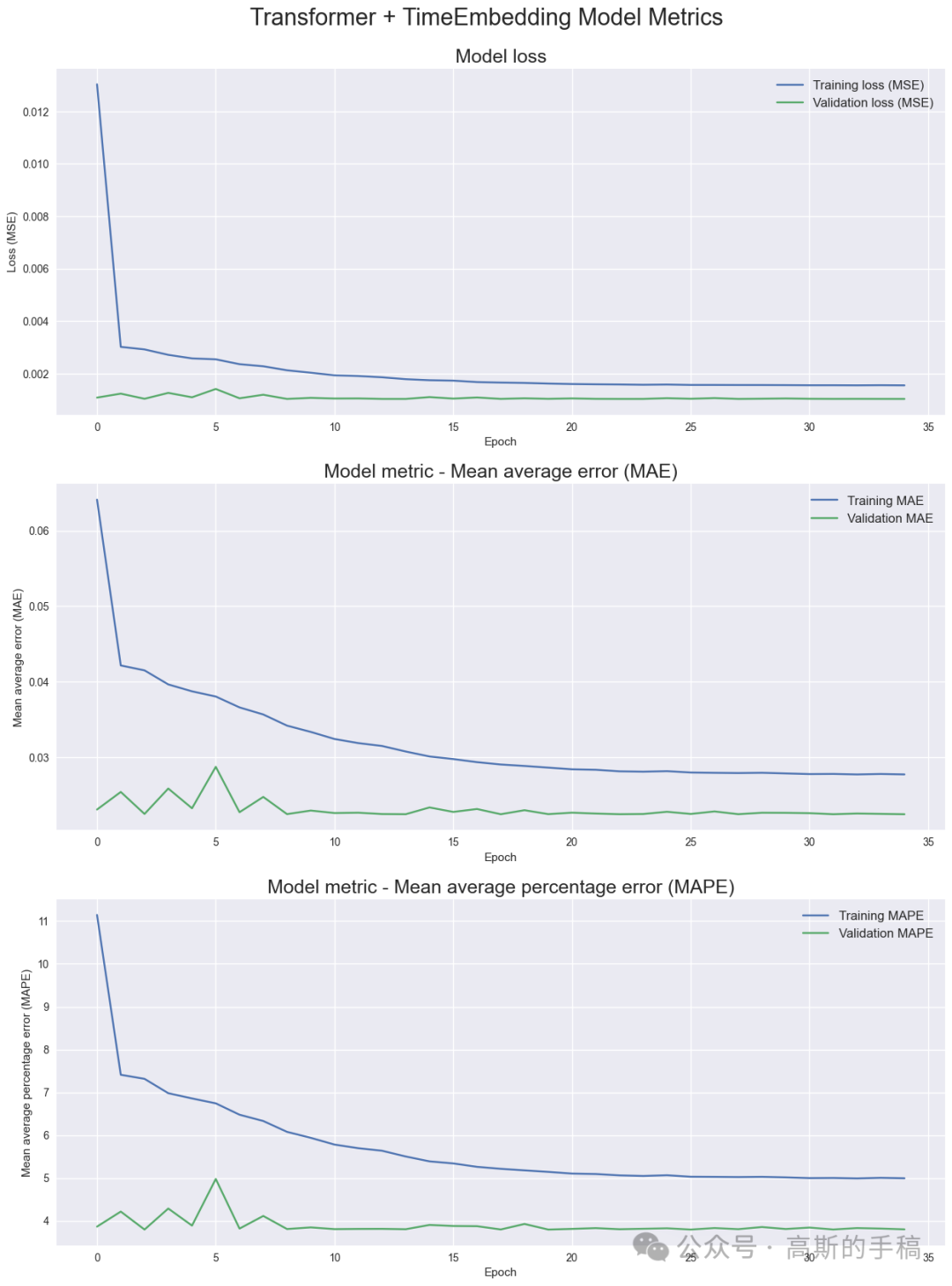
'''Display model metrics'''`` ``fig = plt.figure(figsize=(15,20))``st = fig.suptitle("Transformer + TimeEmbedding Model Metrics", fontsize=22)``st.set_y(0.92)`` ``#Plot model loss``ax1 = fig.add_subplot(311)``ax1.plot(history.history['loss'], label='Training loss (MSE)')``ax1.plot(history.history['val_loss'], label='Validation loss (MSE)')``ax1.set_title("Model loss", fontsize=18)``ax1.set_xlabel('Epoch')``ax1.set_ylabel('Loss (MSE)')``ax1.legend(loc="best", fontsize=12)`` ``#Plot MAE``ax2 = fig.add_subplot(312)``ax2.plot(history.history['mae'], label='Training MAE')``ax2.plot(history.history['val_mae'], label='Validation MAE')``ax2.set_title("Model metric - Mean average error (MAE)", fontsize=18)``ax2.set_xlabel('Epoch')``ax2.set_ylabel('Mean average error (MAE)')``ax2.legend(loc="best", fontsize=12)`` ``#Plot MAPE``ax3 = fig.add_subplot(313)``ax3.plot(history.history['mape'], label='Training MAPE')``ax3.plot(history.history['val_mape'], label='Validation MAPE')``ax3.set_title("Model metric - Mean average percentage error (MAPE)", fontsize=18)``ax3.set_xlabel('Epoch')``ax3.set_ylabel('Mean average percentage error (MAPE)')``ax3.legend(loc="best", fontsize=12)
Model architecture overview
tf.keras.utils.plot_model(` `model,` `to_file="IBM_Transformer+TimeEmbedding.png",` `show_shapes=True,` `show_layer_names=True,` `expand_nested=True,` `dpi=96,)
tf.keras.utils.plot_model(` `model,` `to_file="IBM_Transformer+TimeEmbedding.png",` `show_shapes=True,` `show_layer_names=True,` `expand_nested=True,` `dpi=96,)
Moving Average
Moving Average - Load IBM data again, to apply rolling window
IBM_path = 'IBM.csv'`` ``df = pd.read_csv(IBM_path, delimiter=',', usecols=['Date', 'Open', 'High', 'Low', 'Close', 'Volume'])`` ``# Replace 0 to avoid dividing by 0 later on``df['Volume'].replace(to_replace=0, method='ffill', inplace=True)` `df.sort_values('Date', inplace=True)`` ``# Apply moving average with a window of 10 days to all columns``df[['Open', 'High', 'Low', 'Close', 'Volume']] = df[['Open', 'High', 'Low', 'Close', 'Volume']].rolling(10).mean()` ` ``# Drop all rows with NaN values``df.dropna(how='any', axis=0, inplace=True)` `df.head()

Moving Average - Plot daily IBM closing prices and volume
fig = plt.figure(figsize=(15,10))``st = fig.suptitle("IBM Close Price and Volume", fontsize=20)``st.set_y(0.92)`` ``ax1 = fig.add_subplot(211)``ax1.plot(df['Close'], label='IBM Close Price')``ax1.set_xticks(range(0, df.shape[0], 1464))``ax1.set_xticklabels(df['Date'].loc[::1464])``ax1.set_ylabel('Close Price', fontsize=18)``ax1.legend(loc="upper left", fontsize=12)`` ``ax2 = fig.add_subplot(212)``ax2.plot(df['Volume'], label='IBM Volume')``ax2.set_xticks(range(0, df.shape[0], 1464))``ax2.set_xticklabels(df['Date'].loc[::1464])``ax2.set_ylabel('Volume', fontsize=18)``ax2.legend(loc="upper left", fontsize=12)
如何学习大模型 AI ?
由于新岗位的生产效率,要优于被取代岗位的生产效率,所以实际上整个社会的生产效率是提升的。
但是具体到个人,只能说是:
“最先掌握AI的人,将会比较晚掌握AI的人有竞争优势”。
这句话,放在计算机、互联网、移动互联网的开局时期,都是一样的道理。
我在一线互联网企业工作十余年里,指导过不少同行后辈。帮助很多人得到了学习和成长。
我意识到有很多经验和知识值得分享给大家,也可以通过我们的能力和经验解答大家在人工智能学习中的很多困惑,所以在工作繁忙的情况下还是坚持各种整理和分享。但苦于知识传播途径有限,很多互联网行业朋友无法获得正确的资料得到学习提升,故此将并将重要的AI大模型资料包括AI大模型入门学习思维导图、精品AI大模型学习书籍手册、视频教程、实战学习等录播视频免费分享出来。

第一阶段(10天):初阶应用
该阶段让大家对大模型 AI有一个最前沿的认识,对大模型 AI 的理解超过 95% 的人,可以在相关讨论时发表高级、不跟风、又接地气的见解,别人只会和 AI 聊天,而你能调教 AI,并能用代码将大模型和业务衔接。
- 大模型 AI 能干什么?
- 大模型是怎样获得「智能」的?
- 用好 AI 的核心心法
- 大模型应用业务架构
- 大模型应用技术架构
- 代码示例:向 GPT-3.5 灌入新知识
- 提示工程的意义和核心思想
- Prompt 典型构成
- 指令调优方法论
- 思维链和思维树
- Prompt 攻击和防范
- …
第二阶段(30天):高阶应用
该阶段我们正式进入大模型 AI 进阶实战学习,学会构造私有知识库,扩展 AI 的能力。快速开发一个完整的基于 agent 对话机器人。掌握功能最强的大模型开发框架,抓住最新的技术进展,适合 Python 和 JavaScript 程序员。
- 为什么要做 RAG
- 搭建一个简单的 ChatPDF
- 检索的基础概念
- 什么是向量表示(Embeddings)
- 向量数据库与向量检索
- 基于向量检索的 RAG
- 搭建 RAG 系统的扩展知识
- 混合检索与 RAG-Fusion 简介
- 向量模型本地部署
- …
第三阶段(30天):模型训练
恭喜你,如果学到这里,你基本可以找到一份大模型 AI相关的工作,自己也能训练 GPT 了!通过微调,训练自己的垂直大模型,能独立训练开源多模态大模型,掌握更多技术方案。
到此为止,大概2个月的时间。你已经成为了一名“AI小子”。那么你还想往下探索吗?
- 为什么要做 RAG
- 什么是模型
- 什么是模型训练
- 求解器 & 损失函数简介
- 小实验2:手写一个简单的神经网络并训练它
- 什么是训练/预训练/微调/轻量化微调
- Transformer结构简介
- 轻量化微调
- 实验数据集的构建
- …
第四阶段(20天):商业闭环
对全球大模型从性能、吞吐量、成本等方面有一定的认知,可以在云端和本地等多种环境下部署大模型,找到适合自己的项目/创业方向,做一名被 AI 武装的产品经理。
- 硬件选型
- 带你了解全球大模型
- 使用国产大模型服务
- 搭建 OpenAI 代理
- 热身:基于阿里云 PAI 部署 Stable Diffusion
- 在本地计算机运行大模型
- 大模型的私有化部署
- 基于 vLLM 部署大模型
- 案例:如何优雅地在阿里云私有部署开源大模型
- 部署一套开源 LLM 项目
- 内容安全
- 互联网信息服务算法备案
- …
学习是一个过程,只要学习就会有挑战。天道酬勤,你越努力,就会成为越优秀的自己。
如果你能在15天内完成所有的任务,那你堪称天才。然而,如果你能完成 60-70% 的内容,你就已经开始具备成为一名大模型 AI 的正确特征了。
这份完整版的大模型 AI 学习资料已经上传CSDN,朋友们如果需要可以微信扫描下方CSDN官方认证二维码免费领取【保证100%免费】


 1465
1465

 被折叠的 条评论
为什么被折叠?
被折叠的 条评论
为什么被折叠?
 到【灌水乐园】发言


