


学习记录
1.VIT模型:
encoder模块和一般的bert没有区别,主要是输入时先将图片向量化,转换成embedding的词结构。
(1)patch embedding:将原始二维数据切分,分成多个patch,每个相当于句子中的一个词,然后经过全连接层,将patch压成一个向量。
(2)position embedding:加入tokens的位置信息,为后面自注意计算做准备。并在向量开头加入了class token,便于后面的特征分类。
然后作为输入进入transformer。实现将实验数据详细切分并全部吸收的功效,实现了多层次多角度的特征学习。
transformer后的全连接层,就是一个MLP-head,将输入时的分类向量取出,输出分类类别。
2.最大似然估计(MLE)和最大后验估计(MAP):
(1)MLE:通过最大化参数给定情况下样本的概率分布来找到参数。对数据进行概率建模,得到数据在多大概率上能被分成一类,将P(x|w)最大化。总之就是根据样本数据训练得到分布。
(2)MAP:公式中的P(w|x)参数位置正好和MLE相反,相比MLE多了先验,多了贝叶斯公式的作用。可抽象化简单理解为对数据本身训练得出的数据依赖更小。(这里可能理解有误,有懂的请指正)
- 🍨 本文为🔗365天深度学习训练营 中的学习记录博客
- 🍖 原作者:K同学啊 | 接辅导、项目定制
- 🚀 文章来源:K同学的学习圈子
一、前期准备
1.设置GPU
import torch
import torch.nn as nn
import torchvision.transforms as transforms
import torchvision
from torchvision import transforms, datasets
import os,PIL,pathlib,warnings

warnings.filterwarnings("ignore")             #忽略警告信息

device = torch.device("cuda" if torch.cuda.is_available() else "cpu")
device
device(type=‘cuda’)
2.导入数据
import os,PIL,random,pathlib

data_dir = './P3/'
data_dir = pathlib.Path(data_dir)

data_paths  = list(data_dir.glob('*'))
classeNames = [str(path).split("\\")[1] for path in data_paths]
classeNames
[‘cloudy’, ‘rain’, ‘shine’, ‘sunrise’]
train_transforms = transforms.Compose([
    transforms.Resize([224, 224]),
    transforms.ToTensor(),
    transforms.Normalize(
        mean=[0.485, 0.456, 0.406],
        std=[0.229, 0.224, 0.225])
])

test_transform = transforms.Compose([
    transforms.Resize([224, 224]),
    transforms.ToTensor(),
    transforms.Normalize(
        mean=[0.485, 0.456, 0.406],
        std=[0.229, 0.224, 0.225])
])

total_data = datasets.ImageFolder("./P3/",transform=train_transforms)
total_data
Dataset ImageFolder
Number of datapoints: 1125
Root location: ./P3/
StandardTransform
Transform: Compose(
Resize(size=[224, 224], interpolation=bilinear, max_size=None, antialias=warn)
ToTensor()
Normalize(mean=[0.485, 0.456, 0.406], std=[0.229, 0.224, 0.225])
)
total_data.class_to_idx
total_data.class_to_idx
{‘cloudy’: 0, ‘rain’: 1, ‘shine’: 2, ‘sunrise’: 3}
3.划分数据集
train_size = int(0.8 * len(total_data))
test_size  = len(total_data) - train_size
train_dataset, test_dataset = torch.utils.data.random_split(total_data, [train_size, test_size])
train_dataset, test_dataset
(<torch.utils.data.dataset.Subset at 0x277892f2a30>,
<torch.utils.data.dataset.Subset at 0x27794642be0>)
batch_size = 1
train_dl = torch.utils.data.DataLoader(train_dataset,
                                           batch_size=batch_size,
                                           shuffle=True,
                                           num_workers=1)
test_dl = torch.utils.data.DataLoader(test_dataset,
                                          batch_size=batch_size,
                                          shuffle=True,
                                          num_workers=1)
for X, y in test_dl:
    print("Shape of X [N, C, H, W]: ", X.shape)
    print("Shape of y: ", y.shape, y.dtype)
    break
Shape of X [N, C, H, W]:  torch.Size([1, 3, 224, 224])
Shape of y:  torch.Size([1]) torch.int64
二、搭建包含C3模块的模型
在卷积神经网络中,收缩率(也称为降采样率或比率)是一种技术,用于减少特征图的空间分辨率,从而减少计算量并降低模型的复杂性。收缩率通常用于残差网络(ResNet)中,以解决深度神经网络中的梯度消失和梯度爆炸问题。 在ResNet中,每个残差块通常包含两个卷积层和一个跳跃连接(shortcut)。跳跃连接允许信息直接从一个层跳到另一个层,而无需通过所有其他层。收缩率可以通过减少中间层的输出通道数来实现,从而减少信息传递的数量和复杂性。具体来说,收缩率可以通过在创建卷积层时设置参数s来实现,其中s是一个介于0和1之间的浮点数,表示每个特征图的收缩率。例如,s=0.5表示每个特征图的输出通道数是输入通道数的一半。 收缩率在ResNet中的作用是减少信息传递的数量和复杂性,从而减少计算量并降低模型的复杂性。同时,收缩率还可以帮助模型学习到更抽象的特征,从而提高模型的性能。
1.搭建模型
import torch.nn.functional as F

def autopad(k, p=None): #k是自动填充的核大小,p是填充值,如果没有p,将用k值的一半作为p值。
                          #如果k是一个列表,则p的值是k的每个元素除以2。返回填充值p。
    if p is None:
        p = k // 2 if isinstance(k, int) else [x // 2 for x in k]
    return p

class Conv(nn.Module):
    def __init__(self, c1, c2, k=1, s=1, p=None, g=1, act=True):
        super().__init__()#在初始化方法中,通过super().init()调用父类的初始化方法。
        self.conv = nn.Conv2d(c1, c2, k, s, autopad(k, p), groups=g, bias=False)#参数包括输入通道数c1,输出通道数c2,卷积核大小k,
                                                    #卷积步长s,填充值p(使用autopad函数自动计算),分组数g,是否使用激活函数act。
        self.bn = nn.BatchNorm2d(c2)#在卷积层之后定义一个批量归一化层self.bn。
        self.act = nn.SiLU() if act is True else (act if isinstance(act, nn.Module) else nn.Identity())
                              # 如果act参数为True,则定义一个SiLU激活函数;如果act参数为False或为一个激活函数模块,则使用act参数作为激活函数。
    def forward(self, x):
        return self.act(self.bn(self.conv(x)))

class Bottleneck(nn.Module):
    def __init__(self, c1, c2, shortcut=True, g=1, e=0.6):  #这里收缩率调低了泛化能力强,但是又会使准确率降低
        super().__init__()
        c_ = int(c2 * e) #定义一个中间通道数c_为c2乘以可选的收缩率e。
        self.cv1 = Conv(c1, c_, 1, 1)
        self.cv2 = Conv(c_, c2, 3, 1, g=g)
        self.add = shortcut and c1 == c2#定义一个布尔变量self.add,用于判断是否使用残差连接,即c1等于c2时,shortcut为True。

    def forward(self, x):
        return x + self.cv2(self.cv1(x)) if self.add else self.cv2(self.cv1(x))

class C3(nn.Module):
    def __init__(self, c1, c2, n=1, shortcut=True, g=1, e=0.6):  #跳跃连接(shortcut)。跳跃连接允许信息直接从一个层跳到另一个层,而无需通过所有其他层。
        super().__init__()
        c_ = int(c2 * e)
        self.cv1 = Conv(c1, c_, 1, 1)
        self.cv2 = Conv(c1, c_, 1, 1)
        self.cv3 = Conv(2 * c_, c2, 1) #super().__init__()用于调用父类Bottleneck的构造函数。
                                       #self.cv1、self.cv2和self.cv3分别定义了三个卷积层,它们的参数c1、c2和c_分别是前一层的输出通道数和当前层的输出通道数。
        self.m = nn.Sequential(*(Bottleneck(c_, c_, shortcut, g, e=1.0) for _ in range(n)))

    def forward(self, x):
        return self.cv3(torch.cat((self.m(self.cv1(x)), self.cv2(x)), dim=1))

class model_K(nn.Module):
    def __init__(self):
        super(model_K, self).__init__()

        self.Conv = Conv(3, 32, 3, 2)

        self.C3_1 = C3(32, 64, 3, 2)

        self.classifier = nn.Sequential(
            nn.Linear(in_features=802816, out_features=100),
            nn.ReLU(),
            nn.Linear(in_features=100, out_features=4)
        )

    def forward(self, x):
        x = self.Conv(x)
        x = self.C3_1(x)
        x = torch.flatten(x, start_dim=1)
        x = self.classifier(x)

        return x

device = "cuda" if torch.cuda.is_available() else "cpu"
print("Using {} device".format(device))

model = model_K().to(device)
model
Using cuda device
model_K(
(Conv): Conv(
(conv): Conv2d(3, 32, kernel_size=(3, 3), stride=(2, 2), padding=(1, 1), bias=False)
(bn): BatchNorm2d(32, eps=1e-05, momentum=0.1, affine=True, track_running_stats=True)
(act): SiLU()
)
(C3_1): C3(
(cv1): Conv(
(conv): Conv2d(32, 38, kernel_size=(1, 1), stride=(1, 1), bias=False)
(bn): BatchNorm2d(38, eps=1e-05, momentum=0.1, affine=True, track_running_stats=True)
(act): SiLU()
)
(cv2): Conv(
(conv): Conv2d(32, 38, kernel_size=(1, 1), stride=(1, 1), bias=False)
(bn): BatchNorm2d(38, eps=1e-05, momentum=0.1, affine=True, track_running_stats=True)
(act): SiLU()
)
(cv3): Conv(
(conv): Conv2d(76, 64, kernel_size=(1, 1), stride=(1, 1), bias=False)
(bn): BatchNorm2d(64, eps=1e-05, momentum=0.1, affine=True, track_running_stats=True)
(act): SiLU()
)
(m): Sequential(
(0): Bottleneck(
(cv1): Conv(
(conv): Conv2d(38, 38, kernel_size=(1, 1), stride=(1, 1), bias=False)
(bn): BatchNorm2d(38, eps=1e-05, momentum=0.1, affine=True, track_running_stats=True)
(act): SiLU()
)
(cv2): Conv(
(conv): Conv2d(38, 38, kernel_size=(3, 3), stride=(1, 1), padding=(1, 1), bias=False)
(bn): BatchNorm2d(38, eps=1e-05, momentum=0.1, affine=True, track_running_stats=True)
(act): SiLU()
)
)
(1): Bottleneck(
(cv1): Conv(
(conv): Conv2d(38, 38, kernel_size=(1, 1), stride=(1, 1), bias=False)
(bn): BatchNorm2d(38, eps=1e-05, momentum=0.1, affine=True, track_running_stats=True)
(act): SiLU()
)
(cv2): Conv(
(conv): Conv2d(38, 38, kernel_size=(3, 3), stride=(1, 1), padding=(1, 1), bias=False)
(bn): BatchNorm2d(38, eps=1e-05, momentum=0.1, affine=True, track_running_stats=True)
(act): SiLU()
)
)
(2): Bottleneck(
(cv1): Conv(
(conv): Conv2d(38, 38, kernel_size=(1, 1), stride=(1, 1), bias=False)
(bn): BatchNorm2d(38, eps=1e-05, momentum=0.1, affine=True, track_running_stats=True)
(act): SiLU()
)
(cv2): Conv(
(conv): Conv2d(38, 38, kernel_size=(3, 3), stride=(1, 1), padding=(1, 1), bias=False)
(bn): BatchNorm2d(38, eps=1e-05, momentum=0.1, affine=True, track_running_stats=True)
(act): SiLU()
)
)
)
)
(classifier): Sequential(
(0): Linear(in_features=802816, out_features=100, bias=True)
(1): ReLU()
(2): Linear(in_features=100, out_features=4, bias=True)
)
)
2.查看模型详情
import torchsummary as summary
summary.summary(model, (3, 224, 224))
    Layer (type)               Output Shape         Param #
        Conv2d-1         [-1, 32, 112, 112]             864
   BatchNorm2d-2         [-1, 32, 112, 112]              64
          SiLU-3         [-1, 32, 112, 112]               0
          Conv-4         [-1, 32, 112, 112]               0
        Conv2d-5         [-1, 38, 112, 112]           1,216
   BatchNorm2d-6         [-1, 38, 112, 112]              76
          SiLU-7         [-1, 38, 112, 112]               0
          Conv-8         [-1, 38, 112, 112]               0
        Conv2d-9         [-1, 38, 112, 112]           1,444
  BatchNorm2d-10         [-1, 38, 112, 112]              76
         SiLU-11         [-1, 38, 112, 112]               0
         Conv-12         [-1, 38, 112, 112]               0
       Conv2d-13         [-1, 38, 112, 112]          12,996
  BatchNorm2d-14         [-1, 38, 112, 112]              76
         SiLU-15         [-1, 38, 112, 112]               0
         Conv-16         [-1, 38, 112, 112]               0
   Bottleneck-17         [-1, 38, 112, 112]               0
       Conv2d-18         [-1, 38, 112, 112]           1,444
  BatchNorm2d-19         [-1, 38, 112, 112]              76
         SiLU-20         [-1, 38, 112, 112]               0
         Conv-21         [-1, 38, 112, 112]               0
       Conv2d-22         [-1, 38, 112, 112]          12,996
  BatchNorm2d-23         [-1, 38, 112, 112]              76
         SiLU-24         [-1, 38, 112, 112]               0
         Conv-25         [-1, 38, 112, 112]               0
   Bottleneck-26         [-1, 38, 112, 112]               0
       Conv2d-27         [-1, 38, 112, 112]           1,444
  BatchNorm2d-28         [-1, 38, 112, 112]              76
         SiLU-29         [-1, 38, 112, 112]               0
         Conv-30         [-1, 38, 112, 112]               0
       Conv2d-31         [-1, 38, 112, 112]          12,996
  BatchNorm2d-32         [-1, 38, 112, 112]              76
         SiLU-33         [-1, 38, 112, 112]               0
         Conv-34         [-1, 38, 112, 112]               0
   Bottleneck-35         [-1, 38, 112, 112]               0
       Conv2d-36         [-1, 38, 112, 112]           1,216
  BatchNorm2d-37         [-1, 38, 112, 112]              76
         SiLU-38         [-1, 38, 112, 112]               0
         Conv-39         [-1, 38, 112, 112]               0
       Conv2d-40         [-1, 64, 112, 112]           4,864
  BatchNorm2d-41         [-1, 64, 112, 112]             128
         SiLU-42         [-1, 64, 112, 112]               0
         Conv-43         [-1, 64, 112, 112]               0
           C3-44         [-1, 64, 112, 112]               0
       Linear-45                  [-1, 100]      80,281,700
         ReLU-46                  [-1, 100]               0
       Linear-47                    [-1, 4]             404
Total params: 80,334,384 Trainable params: 80,334,384 Non-trainable
params: 0 Input size (MB): 0.57 Forward/backward pass size (MB):
170.16 Params size (MB): 306.45 Estimated Total Size (MB): 477.19
三、训练模型
1.编写训练函数
def train(dataloader, model, loss_fn, optimizer):
    size = len(dataloader.dataset)
    num_batches = len(dataloader)

    train_loss, train_acc = 0, 0

    for X, y in dataloader:
        X, y = X.to(device), y.to(device)

        pred = model(X)
        loss = loss_fn(pred, y)

        optimizer.zero_grad()
        loss.backward()
        optimizer.step()

        train_acc  += (pred.argmax(1) == y).type(torch.float).sum().item()
        train_loss += loss.item()

    train_acc  /= size
    train_loss /= num_batches

    return train_acc, train_loss
2.编写训练函数
def test (dataloader, model, loss_fn):
    size        = len(dataloader.dataset)
    num_batches = len(dataloader)
    test_loss, test_acc = 0, 0

    with torch.no_grad():
        for imgs, target in dataloader:
            imgs, target = imgs.to(device), target.to(device)

            target_pred = model(imgs)
            loss        = loss_fn(target_pred, target)

            test_loss += loss.item()
            test_acc  += (target_pred.argmax(1) == target).type(torch.float).sum().item()

    test_acc  /= size
    test_loss /= num_batches

    return test_acc, test_loss
3.正式训练
SGD优化器的基本原理是根据梯度下降的原理,通过不断地调整模型参数来最小化损失函数。SGD优化器的更新策略是每次只更新一个样本的参数,然后根据梯度的大小来决定参数的更新方向和步长。
Adam优化器的基本原理是基于动量的梯度下降和自适应学习率的调整。Adam优化器的更新策略是同时更新多个样本的参数,然后根据梯度的大小和动量的大小来决定参数的更新方向和步长。Adam优化器的自适应学习率调整策略是根据梯度的大小来动态地调整学习率,从而使得模型的收敛速度更快。
因此,Adam优化器相比于SGD优化器,具有更好的收敛速度和稳定性,但也需要更多的计算资源。
这是使用Adam优化器的结果
import copy

optimizer  = torch.optim.Adam(model.parameters(), lr= 0.7e-4)
loss_fn    = nn.CrossEntropyLoss()
epochs     = 20

train_loss = []
train_acc  = []
test_loss  = []
test_acc   = []

best_acc = 0

for epoch in range(epochs):

    model.train()
    epoch_train_acc, epoch_train_loss = train(train_dl, model, loss_fn, optimizer)

    model.eval()
    epoch_test_acc, epoch_test_loss = test(test_dl, model, loss_fn)


    if epoch_test_acc > best_acc:
        best_acc   = epoch_test_acc
        best_model = copy.deepcopy(model)

    train_acc.append(epoch_train_acc)
    train_loss.append(epoch_train_loss)
    test_acc.append(epoch_test_acc)
    test_loss.append(epoch_test_loss)


    lr = optimizer.state_dict()['param_groups'][0]['lr']

    template = ('Epoch:{:2d}, Train_acc:{:.1f}%, Train_loss:{:.3f}, Test_acc:{:.1f}%, Test_loss:{:.3f}, Lr:{:.2E}')
    print(template.format(epoch+1, epoch_train_acc*100, epoch_train_loss,
                          epoch_test_acc*100, epoch_test_loss, lr))


PATH = './best_model.pth'
torch.save(model.state_dict(), PATH)

print('Done')
Epoch: 1, Train_acc:72.1%, Train_loss:0.881, Test_acc:45.3%, Test_loss:4.564, Lr:7.00E-05
Epoch: 2, Train_acc:93.3%, Train_loss:0.217, Test_acc:59.6%, Test_loss:7.254, Lr:7.00E-05
Epoch: 3, Train_acc:99.1%, Train_loss:0.026, Test_acc:66.2%, Test_loss:3.237, Lr:7.00E-05
Epoch: 4, Train_acc:99.1%, Train_loss:0.054, Test_acc:36.9%, Test_loss:12.946, Lr:7.00E-05
Epoch: 5, Train_acc:98.3%, Train_loss:0.080, Test_acc:63.6%, Test_loss:10.122, Lr:7.00E-05
Epoch: 6, Train_acc:97.2%, Train_loss:0.124, Test_acc:44.9%, Test_loss:17.192, Lr:7.00E-05
Epoch: 7, Train_acc:98.4%, Train_loss:0.067, Test_acc:57.3%, Test_loss:8.758, Lr:7.00E-05
Epoch: 8, Train_acc:100.0%, Train_loss:0.002, Test_acc:59.6%, Test_loss:8.523, Lr:7.00E-05
Epoch: 9, Train_acc:100.0%, Train_loss:0.000, Test_acc:52.9%, Test_loss:6.308, Lr:7.00E-05
Epoch:10, Train_acc:100.0%, Train_loss:0.000, Test_acc:51.1%, Test_loss:14.270, Lr:7.00E-05
Epoch:11, Train_acc:100.0%, Train_loss:0.000, Test_acc:48.9%, Test_loss:11.451, Lr:7.00E-05
Epoch:12, Train_acc:100.0%, Train_loss:0.000, Test_acc:45.3%, Test_loss:9.089, Lr:7.00E-05
Epoch:13, Train_acc:100.0%, Train_loss:0.000, Test_acc:44.4%, Test_loss:9.411, Lr:7.00E-05
Epoch:14, Train_acc:100.0%, Train_loss:0.000, Test_acc:46.7%, Test_loss:11.623, Lr:7.00E-05
Epoch:15, Train_acc:100.0%, Train_loss:0.000, Test_acc:44.9%, Test_loss:11.957, Lr:7.00E-05
Epoch:16, Train_acc:100.0%, Train_loss:0.000, Test_acc:57.8%, Test_loss:7.548, Lr:7.00E-05
Epoch:17, Train_acc:100.0%, Train_loss:0.000, Test_acc:48.0%, Test_loss:7.625, Lr:7.00E-05
Epoch:18, Train_acc:100.0%, Train_loss:0.000, Test_acc:47.6%, Test_loss:13.050, Lr:7.00E-05
Epoch:19, Train_acc:100.0%, Train_loss:0.000, Test_acc:53.8%, Test_loss:7.652, Lr:7.00E-05
Epoch:20, Train_acc:100.0%, Train_loss:0.000, Test_acc:48.9%, Test_loss:8.773, Lr:7.00E-05
Done
这是SGD优化器的结果
import copy

optimizer  = torch.optim.SGD(model.parameters(), lr= 0.7e-4)
loss_fn    = nn.CrossEntropyLoss()
epochs     = 20

train_loss = []
train_acc  = []
test_loss  = []
test_acc   = []

best_acc = 0

for epoch in range(epochs):

    model.train()
    epoch_train_acc, epoch_train_loss = train(train_dl, model, loss_fn, optimizer)

    model.eval()
    epoch_test_acc, epoch_test_loss = test(test_dl, model, loss_fn)


    if epoch_test_acc > best_acc:
        best_acc   = epoch_test_acc
        best_model = copy.deepcopy(model)

    train_acc.append(epoch_train_acc)
    train_loss.append(epoch_train_loss)
    test_acc.append(epoch_test_acc)
    test_loss.append(epoch_test_loss)


    lr = optimizer.state_dict()['param_groups'][0]['lr']

    template = ('Epoch:{:2d}, Train_acc:{:.1f}%, Train_loss:{:.3f}, Test_acc:{:.1f}%, Test_loss:{:.3f}, Lr:{:.2E}')
    print(template.format(epoch+1, epoch_train_acc*100, epoch_train_loss,
                          epoch_test_acc*100, epoch_test_loss, lr))


PATH = './best_model.pth'
torch.save(model.state_dict(), PATH)

print('Done')
Epoch: 1, Train_acc:76.9%, Train_loss:0.603, Test_acc:43.1%, Test_loss:2.579, Lr:7.00E-05
Epoch: 2, Train_acc:98.9%, Train_loss:0.079, Test_acc:28.9%, Test_loss:6.187, Lr:7.00E-05
Epoch: 3, Train_acc:100.0%, Train_loss:0.026, Test_acc:41.3%, Test_loss:3.137, Lr:7.00E-05
Epoch: 4, Train_acc:100.0%, Train_loss:0.014, Test_acc:40.9%, Test_loss:2.898, Lr:7.00E-05
Epoch: 5, Train_acc:100.0%, Train_loss:0.011, Test_acc:43.6%, Test_loss:3.023, Lr:7.00E-05
Epoch: 6, Train_acc:100.0%, Train_loss:0.008, Test_acc:38.2%, Test_loss:3.117, Lr:7.00E-05
Epoch: 7, Train_acc:100.0%, Train_loss:0.007, Test_acc:41.8%, Test_loss:4.132, Lr:7.00E-05
Epoch: 8, Train_acc:100.0%, Train_loss:0.006, Test_acc:37.3%, Test_loss:4.899, Lr:7.00E-05
Epoch: 9, Train_acc:100.0%, Train_loss:0.005, Test_acc:42.2%, Test_loss:3.136, Lr:7.00E-05
Epoch:10, Train_acc:100.0%, Train_loss:0.005, Test_acc:35.6%, Test_loss:4.537, Lr:7.00E-05
Epoch:11, Train_acc:100.0%, Train_loss:0.004, Test_acc:42.7%, Test_loss:3.710, Lr:7.00E-05
Epoch:12, Train_acc:100.0%, Train_loss:0.004, Test_acc:36.9%, Test_loss:5.370, Lr:7.00E-05
Epoch:13, Train_acc:100.0%, Train_loss:0.004, Test_acc:48.4%, Test_loss:2.399, Lr:7.00E-05
Epoch:14, Train_acc:100.0%, Train_loss:0.003, Test_acc:41.3%, Test_loss:3.345, Lr:7.00E-05
Epoch:15, Train_acc:100.0%, Train_loss:0.003, Test_acc:40.9%, Test_loss:3.509, Lr:7.00E-05
Epoch:16, Train_acc:100.0%, Train_loss:0.003, Test_acc:44.4%, Test_loss:2.837, Lr:7.00E-05
Epoch:17, Train_acc:100.0%, Train_loss:0.003, Test_acc:38.7%, Test_loss:5.496, Lr:7.00E-05
Epoch:18, Train_acc:100.0%, Train_loss:0.002, Test_acc:36.4%, Test_loss:4.491, Lr:7.00E-05
Epoch:19, Train_acc:100.0%, Train_loss:0.002, Test_acc:42.7%, Test_loss:2.772, Lr:7.00E-05
Epoch:20, Train_acc:100.0%, Train_loss:0.002, Test_acc:35.1%, Test_loss:5.278, Lr:7.00E-05
Done
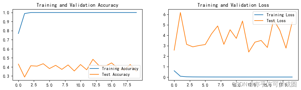
四、结果可视化
1.Loss和Acurracy图
import matplotlib.pyplot as plt
#隐藏警告
import warnings
warnings.filterwarnings("ignore")
plt.rcParams['font.sans-serif']    = ['SimHei'] # 用来正常显示中文标签
plt.rcParams['axes.unicode_minus'] = False      # 用来正常显示负号
plt.rcParams['figure.dpi']         = 100        #分辨率

epochs_range = range(epochs)

plt.figure(figsize=(12, 3))
plt.subplot(1, 2, 1)

plt.plot(epochs_range, train_acc, label='Training Accuracy')
plt.plot(epochs_range, test_acc, label='Test Accuracy')
plt.legend(loc='lower right')
plt.title('Training and Validation Accuracy')

plt.subplot(1, 2, 2)
plt.plot(epochs_range, train_loss, label='Training Loss')
plt.plot(epochs_range, test_loss, label='Test Loss')
plt.legend(loc='upper right')
plt.title('Training and Validation Loss')
plt.show()
best_model.eval()
epoch_test_acc, epoch_test_loss = test(test_dl, best_model, loss_fn)
epoch_test_acc, epoch_test_loss
(0.48444444444444446, 2.399209665327362)
epoch_test_acc
0.48444444444444446


 408
408


 被折叠的 条评论
为什么被折叠?
被折叠的 条评论
为什么被折叠?
 到【灌水乐园】发言


