


供个人查询
文章目录
- methods of KGE & logical rules
- 1. Injecting Logical Background Knowledge into Embeddings for Relation Extraction
- 2. KALE: Jointly Embedding Knowledge Graphs and Logical Rules
- 3. Logic Rules Powered Knowledge Graph Embedding
- 粗略比较1,2,3
- 4. Dismult:EMBEDDING ENTITIES AND RELATIONS FOR LEARN- ING AND INFERENCE IN KNOWLEDGE BASES
- 5. IterE: Iteratively Learning Embeddings and Rules for Knowledge Graph Reasoning
- methods of rule mining
methods of KGE & logical rules
1. Injecting Logical Background Knowledge into Embeddings for Relation Extraction
2015, NAACL, Tim Rockta ̈schel
pdf:https://rockt.github.io/pdf/rocktaschel2015injecting.pdf
github:https://github.com/uclnlp/low-rank-logic
开放领域关系抽取问题。
模型
整个模型框架如下:

- 矩阵分解部分
具体来说,用 binary matrix
∣
P
∣
×
∣
R
∣
|P|\times |\mathcal{R}|
∣P∣×∣R∣的每一行表示constant-pairs,每一列是predicates,通过矩阵分解的方式可以得到两个embeddings,
∣
P
∣
×
k
|P|\times k
∣P∣×k 和
k
×
∣
R
∣
k \times |\mathcal{R}|
k×∣R∣,分别表示constant-pairs embeddings
v
e
i
,
e
j
v_{e_i,e_j}
vei,ej 和 predicate embeddings
v
r
m
v_{r_m}
vrm。矩阵中存的内容参考Riedel 2013(可以大致看这篇):
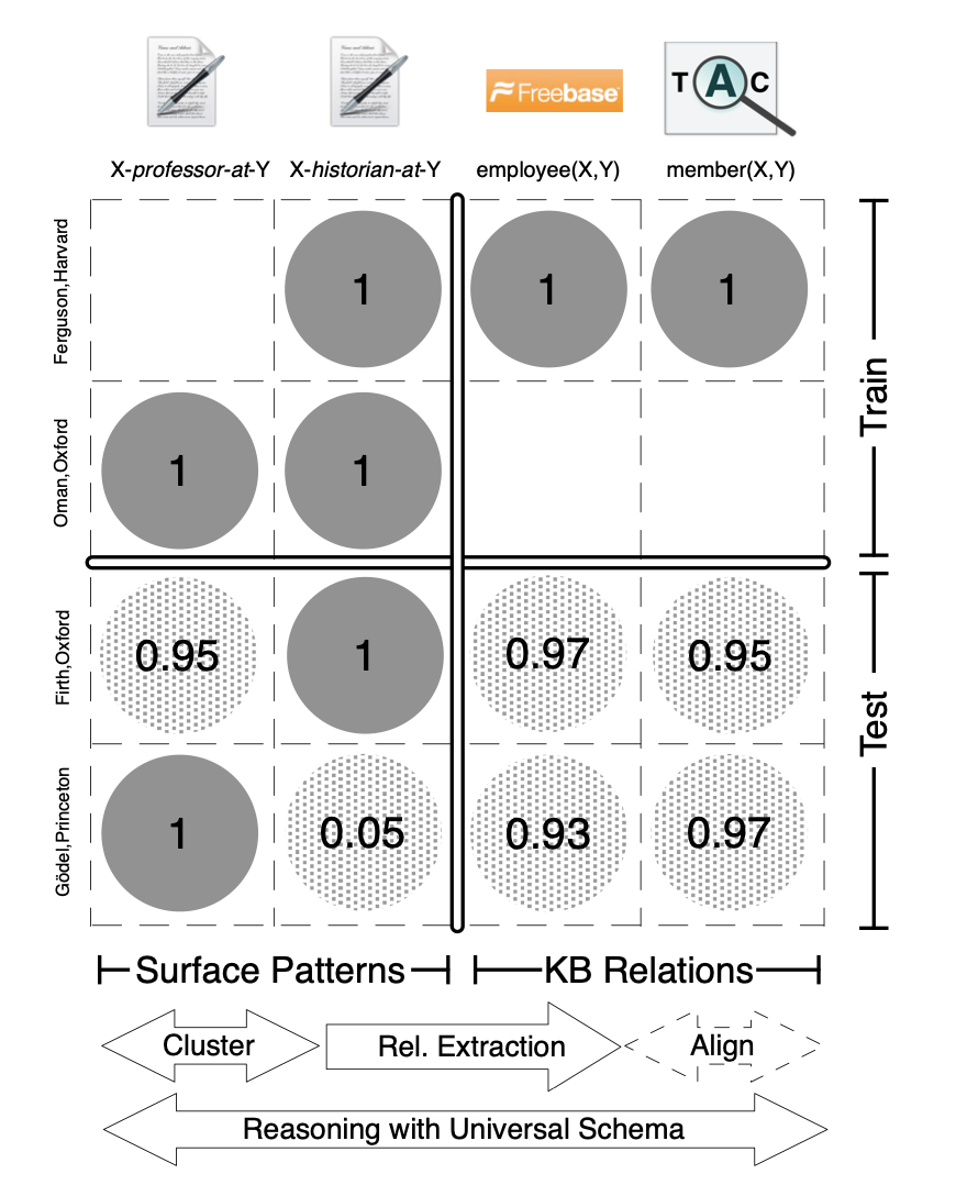
已知embeddings V V V的情况下,对于已知事实 w w w,可以定义如下的概率分布。其中, π m e i , e j = σ ( v r m , v e i , e j ) \pi_m^{e_i,e_j}= \sigma (v_{r_m},v_{e_i,e_j}) πmei,ej=σ(vrm,vei,ej), v ( ⋅ ) v_{(\cdot)} v(⋅)表示对应的embedding,可以通过最大化本公式得到。
p ( w ∣ V ) = ∏ r m ( e i , e j ) ∈ w π m e i , e j ∏ r m ( e i , e j ) ∉ w ( 1 − π m e i , e j ) p(\mathbf{w} | \mathbf{V})=\prod_{r_{m}\left(e_{i}, e_{j}\right) \in w} \pi_{m}^{e_{i}, e_{j}} \prod_{r_{m}\left(e_{i}, e_{j}\right) \notin w}\left(1-\pi_{m}^{e_{i}, e_{j}}\right) p(w∣V)=rm(ei,ej)∈w∏πmei,ejrm(ei,ej)∈/w∏(1−πmei,ej)
- 融入规则部分,包括两种方式
-
Pre-Factorization Inference:通过已经抽取到的规则生成新的三元组,将新三元组加入,产生新的规则,继续训练得到规则,再产生三元组,反复直到没有新的三元组产生。
-
joint 模型:训练的整体目标为:
min v ∑ F ∈ z ~ L ( [ F ] ) \min _{\mathbf{v}} \sum_{\mathcal{F} \in \tilde{\mathbf{z}}} \mathcal{L}([\mathcal{F}]) vminF∈z~∑L([F])对于facts, [ F ] [\mathcal{F}] [F]是 p ( w ∣ V ) p(\mathbf{w} | \mathbf{V}) p(w∣V)的marginal probability , L ( [ F ] ) : = − log ( [ F ] ) \mathcal{L}([\mathcal{F}]):=-\log ([\mathcal{F}]) L([F]):=−log([F])
对于logic formulae,遵循了product t-norm,即 [ A ∧ B ] [\mathcal{A} \wedge \mathcal{B}] [A∧B]的边缘概率可以用 [ A ] [ B ] [\mathcal{A}][\mathcal{B}] [A][B]计算, 其他如下:
针对的是KGC: "predict hidden knowledge-base relations from observed natural- language relations. "
2. KALE: Jointly Embedding Knowledge Graphs and Logical Rules
Shu Guo、Quan Wang
EMNLP 2016:https://www.aclweb.org/anthology/D16-1019.pdf
Wang(2015) 和 Wei(2015)利用KGE和rules去做KGC的任务,采用的pipline的方式;Rockta ̈schel(2015)采用joint模型将一阶逻辑规则注入到KGE过程中,因为它关注的是关系抽取项目,是实体对而非单个实体创建embedding,因此没有办法处理单个实体。
本文介绍了KALE(entity and relation Embeddings by jointly modeling Knowledge And Logic.)
之前的模型通常在马尔可夫逻辑网络的基础上,对知识获取和推理中的逻辑规则进行了广泛的研究(Richardson和Domingos,2006;Bröcheler等,2010; Pujara等,2013; Beltagy和Mooney, 2014)。最近,人们对组合逻辑规则和嵌入模型越来越感兴趣。
模型

KG embedding
I
(
e
i
,
r
k
,
e
j
)
=
1
−
1
3
d
∥
e
i
+
r
k
−
e
j
∥
1
I\left(e_{i}, r_{k}, e_{j}\right)=1-\frac{1}{3 \sqrt{d}}\left\|\mathbf{e}_{i}+\mathbf{r}_{k}-\mathbf{e}_{j}\right\|_{1}
I(ei,rk,ej)=1−3d1∥ei+rk−ej∥1
得分位于[0,1] 区间指示the truth value of that triple.
rule modeling
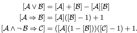
采用t-norm fuzzy logics,它将复杂公式的真值定义为其成分的真值的组合。本文遵循Bröcheler的定义采用product t-norm,对逻辑规则的组合定义如下:
I
(
f
1
∧
f
2
)
=
I
(
f
1
)
⋅
I
(
f
2
)
I
(
f
1
∨
f
2
)
=
I
(
f
1
)
+
I
(
f
2
)
−
I
(
f
1
)
⋅
I
(
f
2
)
I
(
¬
f
1
)
=
1
−
I
(
f
1
)
\begin{aligned} I\left(f_{1} \wedge f_{2}\right) &=I\left(f_{1}\right) \cdot I\left(f_{2}\right) \\ I\left(f_{1} \vee f_{2}\right) &=I\left(f_{1}\right)+I\left(f_{2}\right)-I\left(f_{1}\right) \cdot I\left(f_{2}\right) \\ I\left(\neg f_{1}\right) &=1-I\left(f_{1}\right) \end{aligned}
I(f1∧f2)I(f1∨f2)I(¬f1)=I(f1)⋅I(f2)=I(f1)+I(f2)−I(f1)⋅I(f2)=1−I(f1)
可以推演出:
I
(
¬
f
1
∧
f
2
)
=
I
(
f
2
)
−
I
(
f
1
)
⋅
I
(
f
2
)
I
(
f
1
⇒
f
2
)
=
I
(
f
1
)
⋅
I
(
f
2
)
−
I
(
f
1
)
+
1
\begin{array}{l}{I\left(\neg f_{1} \wedge f_{2}\right)=I\left(f_{2}\right)-I\left(f_{1}\right) \cdot I\left(f_{2}\right)} \\ {I\left(f_{1} \Rightarrow f_{2}\right)=I\left(f_{1}\right) \cdot I\left(f_{2}\right)-I\left(f_{1}\right)+1}\end{array}
I(¬f1∧f2)=I(f2)−I(f1)⋅I(f2)I(f1⇒f2)=I(f1)⋅I(f2)−I(f1)+1
对$f \triangleq\left(e_{m}, r_{s}, e_{n}\right) \Rightarrow\left(e_{m}, r_{t}, e_{n}\right)$有:
I
(
f
)
=
I
(
e
m
,
r
s
,
e
n
)
⋅
I
(
e
m
,
r
t
,
e
n
)
−
I
(
e
m
,
r
s
,
e
n
)
+
1
\begin{aligned} I(f) &=I\left(e_{m}, r_{s}, e_{n}\right) \cdot I\left(e_{m}, r_{t}, e_{n}\right) \\ &-I\left(e_{m}, r_{s}, e_{n}\right)+1 \end{aligned}
I(f)=I(em,rs,en)⋅I(em,rt,en)−I(em,rs,en)+1
对
f
≜
(
e
ℓ
,
r
s
1
,
e
m
)
∧
(
e
m
,
r
s
2
,
e
n
)
⇒
(
e
ℓ
,
r
t
,
e
n
)
f \triangleq\left(e_{\ell}, r_{s_{1}}, e_{m}\right) \wedge\left(e_{m}, r_{s_{2}}, e_{n}\right) \Rightarrow\left(e_{\ell}, r_{t}, e_{n}\right)
f≜(eℓ,rs1,em)∧(em,rs2,en)⇒(eℓ,rt,en)有:
I
(
f
)
=
I
(
e
ℓ
,
r
s
1
,
e
m
)
⋅
I
(
e
m
,
r
s
2
,
e
n
)
⋅
I
(
e
ℓ
,
r
t
,
e
n
)
−
I
(
e
ℓ
,
r
s
1
,
e
m
)
⋅
I
(
e
m
,
r
s
2
,
e
n
)
+
1
\begin{aligned} I(f) &=I\left(e_{\ell}, r_{s_{1}}, e_{m}\right) \cdot I\left(e_{m}, r_{s_{2}}, e_{n}\right) \cdot I\left(e_{\ell}, r_{t}, e_{n}\right) \\ &-I\left(e_{\ell}, r_{s_{1}}, e_{m}\right) \cdot I\left(e_{m}, r_{s_{2}}, e_{n}\right)+1 \end{aligned}
I(f)=I(eℓ,rs1,em)⋅I(em,rs2,en)⋅I(eℓ,rt,en)−I(eℓ,rs1,em)⋅I(em,rs2,en)+1
The larger the truth values are, the better the ground rules are satisfied.
联合训练
训练集合包括了两个部分,1)KG中的三元组,2)ground rules,损失函数定义如下
min
{
e
}
,
{
r
}
∑
f
+
∈
F
∑
f
−
∈
N
f
+
[
γ
−
I
(
f
+
)
+
I
(
f
−
)
]
+
s.t.
∥
e
∥
2
≤
1
,
∀
e
∈
E
;
∥
r
∥
2
≤
1
,
∀
r
∈
R
\begin{array}{c}{\min _{\{\mathbf{e}\},\{\mathbf{r}\}} \sum_{f^{+} \in \mathcal{F}} \sum_{f^{-} \in \mathcal{N}_{f^{+}}}\left[\gamma-I\left(f^{+}\right)+I\left(f^{-}\right)\right]_{+}} \\ {\text {s.t. }\|\mathbf{e}\|_{2} \leq 1, \forall e \in \mathcal{E} ;\|\mathbf{r}\|_{2} \leq 1, \forall r \in \mathcal{R}}\end{array}
min{e},{r}∑f+∈F∑f−∈Nf+[γ−I(f+)+I(f−)]+s.t. ∥e∥2≤1,∀e∈E;∥r∥2≤1,∀r∈R
这里的 f f f就是上面两个部分,负样本的的产生分为两步。对KG中的三元组,随机替换头尾实体作为负样本,对于ground rules,随机替换其中的关系作为负样本,比如对( Paris, Capital-Of, France) ⇒(Paris, Located-In, France ),可能生成的负样本为 (Paris,Capital-Of,France)⇒ (Paris,Has-Spouse,France)。
实验
在wordnet上和FB上级行了链接预测和三元组分类任务。
(这里的逻辑规则或者是手动获得或者是自动抽取获得)构建规则的方式:首先运行TransE模块,之后用公式(2)(3)计算得分,对其排序并手动选择top,最终在WN上确定了14条规则,在FB上确定了47条规则。
3. Logic Rules Powered Knowledge Graph Embedding
arxiv 2019:https://arxiv.org/pdf/1903.03772.pdf
总结了之前工作的缺点是:
1) 大多数知识图嵌入模型未充分利用逻辑规则怎么证明?
2)手动选择使用的规则
3)规则以真值的形式编码,导致了一对多映射的映射。文中没有看到更多说明?
4)逻辑符号的代数运算在三元组和规则中不一致。感觉本质跟KALE差不多?
文章的贡献:
1)提出一种规则增强的方法,可以和任何Traslation based Embedding method 集成。
2)介绍了一种自动挖掘规则(三种类型的规则)并给出置信度(大概是通过规则产生的triples中facts占据所有产生的triples的比例)
3)将triples和logical rules transform到the same first-order logical space(将facts表示为
h
(
r
)
⇒
t
h(r)\Rightarrow t
h(r)⇒t)
4)在 filtered Hit@1上效果提升显著
方法
RULE EXTRACTION
主要针对三种规则:
- inference rule: ∀ h , t : ( h , r 1 , t ) ⇒ ( h , r 2 , t ) \forall h, t:\left(h, r_{1}, t\right) \Rightarrow\left(h, r_{2}, t\right) ∀h,t:(h,r1,t)⇒(h,r2,t),如 ( W a s h i n g t o n , i s C a p i t a l o f , U S A ) ⇒ ( W a s h i n g t o n , i s L o c a t e d i n , U S A ) (Washington, isCapitalof, USA)⇒(Washington, isLocatedin, USA) (Washington,isCapitalof,USA)⇒(Washington,isLocatedin,USA)
- transitivity rule
- antisymmetryrule: ∀ h , t : ( h , r 1 , t ) ⇔ ( t , r 2 , h ) \forall h, t:\left(h, r_{1}, t\right) \Leftrightarrow\left(t, r_{2}, h\right) ∀h,t:(h,r1,t)⇔(t,r2,h)
整体的抽取流程如图:

-
Rule Sample Extraction。结合上图理解。
-
Rule Candidate Extraction
这里需要注意的是:对于inference rule文中有详细说明怎么区分concept和instance,主要是利用probase得到the concept of an entity,如下图:
Relation Concept-Instance Pairs location.country ( location-country ) people. profession ( people-profession ) music. songwriter ( music-songwriter ) sports.boxer ( sports-boxer ) book. magazine ( book-magazine ) \begin{array}{ll}\hline \text { Relation } & {\text { Concept-Instance Pairs }} \\ \hline \text { location.country } & {(\text { location-country })} \\ {\text { people. profession }} & {(\text { people-profession })} \\ {\text { music. songwriter }} & {(\text { music-songwriter })} \\ {\text { sports.boxer }} & {(\text { sports-boxer })} \\ {\text { book. magazine }} & {(\text { book-magazine })} \\ \hline\end{array} Relation location.country people. profession music. songwriter sports.boxer book. magazine Concept-Instance Pairs ( location-country )( people-profession )( music-songwriter )( sports-boxer )( book-magazine )
从上图中可以看到country是location的instance,(这里的Relation对应上面说的entity的concept)。
FB中的relation是有层次结构的,如 /location/country/capital 和 /location/location/contains ,为了在inference rule中这两个谁是concept/instance,可以利用上面提到的the concept of entity。 -
Score Calculation
在KALE中,排名靠前的规则是通过手动过滤的,很难在large-scale KG上应用,因此,本文提出一个从候选池中自动选择规则的方法。score计算过程如下。 G e t N e w t r i p l e s ( ) GetNewtriples() GetNewtriples()用来生成新的三元组,对 ( h , r 1 , t ) (h,r_1,t) (h,r1,t)用Inference candidate rule r 1 ⇒ r 2 r_1 \Rightarrow r_2 r1⇒r2,能够生成 ( h , r 2 , t ) (h,r_2,t) (h,r2,t)这样的new triple

RULE-ENHANCED KNOWLEDGE GRAPH EMBEDDING
- Rule-Enhanced TransE Model
s 1 ( h , r , t ) = ∥ h + r − t ∥ l / 2 s_{1}(h, r, t)=\|\mathbf{h}+\mathbf{r}-\mathbf{t}\|_{l / 2} s1(h,r,t)=∥h+r−t∥l/2
下图是逻辑规则对应的数学表示:
First-order logic Mathematical expression r ( h ) r + h a ⇒ b a − b h ∈ C h ⋅ C ( C is a matrix ) a ∧ b a ⊗ b a ⇔ b ( a − b ) ⊗ ( a − b ) \begin{array}{ll}\hline \text { First-order logic } & {\text { Mathematical expression }} \\ \hline r(h) & {\mathbf{r}+\mathbf{h}} \\ {a \Rightarrow b} & {\mathbf{a}-\mathbf{b}} \\ {h \in C} & {\mathbf{h} \cdot \mathbf{C}(\mathbf{C} \text { is a matrix })} \\ {a \wedge b} & {\mathbf{a} \otimes \mathbf{b}} \\ {a \Leftrightarrow b} & {(\mathbf{a}-\mathbf{b}) \otimes(\mathbf{a}-\mathbf{b})} \\ \hline\end{array} First-order logic r(h)a⇒bh∈Ca∧ba⇔b Mathematical expression r+ha−bh⋅C(C is a matrix )a⊗b(a−b)⊗(a−b)
用上面的对应表示,三种类型的规则有以下转换:
Inference rule
s 2 ( f ) = ∥ ( h m ⋅ C ) ⊗ ( h m + r 1 − t n ) − ( h m + r 2 − t n ) ∥ l 1 / 2 s_{2}(f)=\left\|\left(\mathbf{h}_{m} \cdot \mathbf{C}\right) \otimes\left(\mathbf{h}_{m}+\mathbf{r}_{1}-\mathbf{t}_{n}\right)-\left(\mathbf{h}_{m}+\mathbf{r}_{2}-\mathbf{t}_{n}\right)\right\|_{l_{1 / 2}} s2(f)=∥(hm⋅C)⊗(hm+r1−tn)−(hm+r2−tn)∥l1/2
Transitivity rule
s 3 ( f ) = ∥ [ ( e l + r 1 − e m ) ⊗ ( e m + r 2 − e n ) ] − ( e l + r 3 − e n ) ∥ l 1 / 2 \begin{aligned} s_{3}(f)=& \|\left[\left(\mathbf{e}_{l}+\mathbf{r}_{1}-\mathbf{e}_{m}\right) \otimes\left(\mathbf{e}_{m}+\mathbf{r}_{2}-\mathbf{e}_{n}\right)\right] \\ &-\left(\mathbf{e}_{l}+\mathbf{r}_{3}-\mathbf{e}_{n}\right) \|_{l_{1 / 2}} \end{aligned} s3(f)=∥[(el+r1−em)⊗(em+r2−en)]−(el+r3−en)∥l1/2
Antisymmetry rule
s 4 ( f ) = ∥ ( T R f − T R b ) ⊗ ( T R b − T R f ) ∥ l 1 / 2 T R f = h m + r 1 − t n , T R b = t n + r 2 − h m \begin{aligned} s_{4}(f) &=\left\|\left(\mathrm{TR}_{f}-\mathrm{TR}_{b}\right) \otimes\left(\mathrm{TR}_{b}-\mathrm{TR}_{f}\right)\right\|_{l_{1 / 2}} \\ \mathrm{TR}_{f} &=\mathrm{h}_{m}+\mathrm{r}_{1}-\mathrm{t}_{n}, \quad \mathrm{TR}_{b}=\mathrm{t}_{n}+\mathrm{r}_{2}-\mathrm{h}_{m} \end{aligned} s4(f)TRf=∥(TRf−TRb)⊗(TRb−TRf)∥l1/2=hm+r1−tn,TRb=tn+r2−hm - Rule-Enhanced TransH Model,同上过程,具体看原文
- Rule-Enhanced TransR Model,同上过程,具体看原文
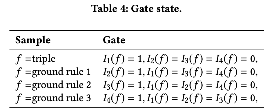
GLOBAL OBJECTIVE FUNCTION

I n ( f ) I_n(f) In(f)表示了门,如下图所示
实验
Datasets
FB166,FB15k,WN18
Dataset
#
E
#
R
#
Trip. (Train
/
Valid
/
Test)
FB15K
14
,
951
1
,
345
483
,
142
50
,
000
59
,
071
F
B
166
9
,
658
166
100
,
289
10
,
457
12
,
327
W
N
18
40
,
943
18
141
,
442
5
,
000
5
,
000
\begin{array}{cccccc}\hline \text { Dataset } & {\# \mathrm{E}} & {\# \mathrm{R}} & \# \text { Trip. (Train } &/ \text { Valid } &/ \text { Test) } \\ \hline \text { FB15K } & {14,951} & {1,345} & {483,142} & {50,000} & {59,071} \\ {\mathrm{FB} 166} & {9,658} & {166} & {100,289} & {10,457} & {12,327} \\ {\mathrm{WN} 18} & {40,943} & {18} & {141,442} & {5,000} & {5,000} \\ \hline\end{array}
Dataset FB15K FB166WN18#E14,9519,65840,943#R1,34516618# Trip. (Train 483,142100,289141,442/ Valid 50,00010,4575,000/ Test) 59,07112,3275,000
指标
- MR,mean rank,越小越好
M R = 1 2 # K t ∑ i = 1 # K t ( r a n k i h + r a n k i t ) M R=\frac{1}{2 \# \mathcal{K}_{t}} \sum_{i=1}^{\# \mathcal{K}_{t}}\left(r a n k_{i h}+r a n k_{i t}\right) MR=2#Kt1i=1∑#Kt(rankih+rankit) - MRR,mean reciprocal rank,平均导数排名,越大越好。
M R R = 1 2 # K t ∑ i = 1 # ( 1 r a n k i h + 1 r a n k i t ) M R R=\frac{1}{2 \# \mathcal{K}_{t}} \sum_{i=1}^{\#}\left(\frac{1}{r a n k_{i h}}+\frac{1}{r a n k_{i t}}\right) MRR=2#Kt1i=1∑#(rankih1+rankit1) - Hits@n
Hits @ n = 1 2 ∗ K t ∑ j = 1 # K t ( I n ( r a n k i h ) + I n ( rank i t ) ) I n ( rank i ) = { 1 if r a n k i ≤ n 0 otherwise \text {Hits} @ n=\frac{1}{2 * \mathcal{K}_{t}} \sum_{j=1}^{\# \mathcal{K}_{t}}\left(I_{n}\left(r a n k_{i h}\right)+I_{n}\left(\text {rank}_{i t}\right)\right)\\ I_{n}\left(\operatorname{rank}_{i}\right)=\left\{\begin{array}{ll}{1} & {\text { if } r a n k_{i} \leq n} \\ {0} & {\text { otherwise }}\end{array}\right. Hits@n=2∗Kt1j=1∑#Kt(In(rankih)+In(rankit))In(ranki)={10 if ranki≤n otherwise
Link Prediction
如下是在FB15上的结果,其余数据集上的参考论文。TransE是原始的训练集训练,TransE(Pre)中是将规则得到的new triples加入到训练集中训练,TransE(RUle)是文中提到的将三元组和规则都transform到logical rule space进行joint训练训练。可以看到无论是基于哪种Translation-based model,本文方法的效果都最好。

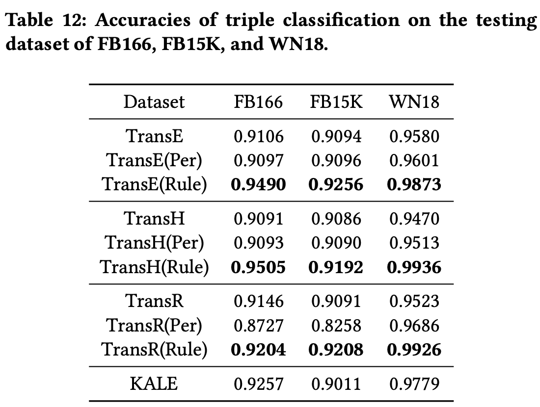
Triple Classification
Triple Classification任务是判断给定的三元组
(
h
,
r
,
t
)
(h,r,t)
(h,r,t)是否正确。
KALE基于TransE。基于TransE,三个数据集上acc提升约1%~2%。
粗略比较1,2,3
-
1 injecting xxx做的是关系抽取任务 不像是现在常见的KGC的任务,更侧重KGC,矩阵分解的办法去进行的,融合规则的方式有两种,一种是将规则产生的三原则加入到训练中,一种是joint的方式,将规则以t-norm的形式加入到矩阵分解过程中。学习到的是实体对和关系的表示。规则也是提前生成。
-
2 KALE受到上面的启发,在TransE模型中加入了规则,加入的方式也是t-norm,joint训练时候的损失函数跟TransE一致,对规则也生成了负样本。学习到实体和关系的表示。规则提前生成。
-
3 powerd xxx这篇规则并非通过手动选择,而是通过度量规则生成的facts中true facts in raw KG的比例来选择,提出可以集成到任何Translate-based KGE方法中。学习到实体和关系的表示。
4. Dismult:EMBEDDING ENTITIES AND RELATIONS FOR LEARN- ING AND INFERENCE IN KNOWLEDGE BASES
ICLR 2015,BiShan Yang, EMBEDDING ENTITIES AND RELATIONS FOR LEARN- ING AND INFERENCE IN KNOWLEDGE BASES
5. IterE: Iteratively Learning Embeddings and Rules for Knowledge Graph Reasoning
2019 IW3C2:paper
methods of rule mining
1. Neural LP: Differentiable learning of logical rules for knowledge base reasoning
NIPS 2017: https://papers.nips.cc/paper/6826-differentiable-learning-of-logical-rules-for-knowledge-base-reasoning.pdf
可直接参考:
文章的研究 probabilistic first-order logical rules for knowledge base reasoning,任务的难点是需要学习连续空间的参数和离散空间的结构。为此,文中提出了一个基于端到端的可微分模型(end-to-end differentiable model),Neural Logic Programming,简称Neural LP。方法基于Tensorlog提出,Tensorlog可以将推理任务编译为可微分操作的序列。
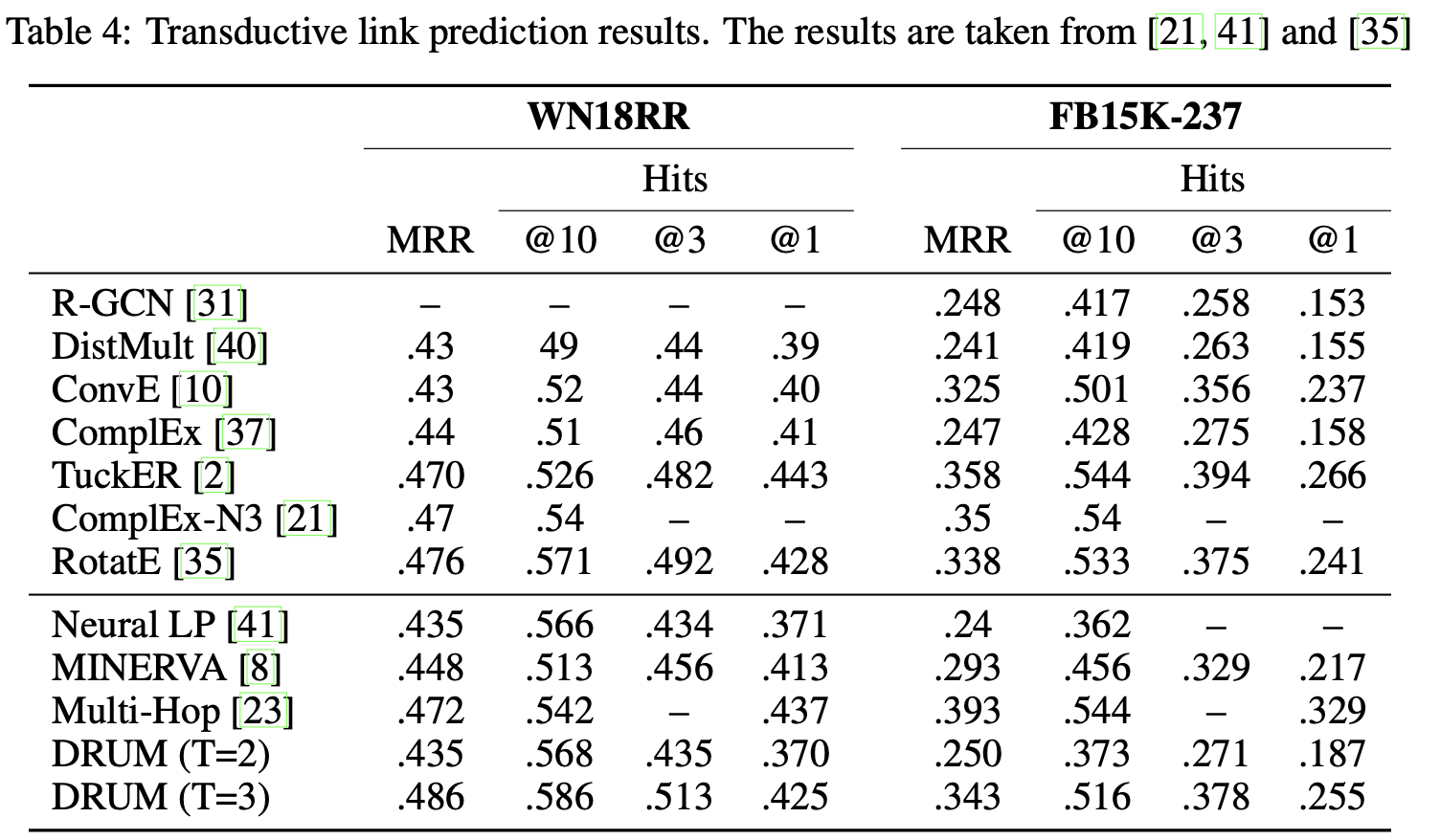
2. DRUM: End-To-End Differentiable Rule Mining On Knowledge Graphs
NeurIPS 2019:https://papers.nips.cc/paper/9669-drum-end-to-end-differentiable-rule-mining-on-knowledge-graphs.pdf
文章的开头就提到说虽然inductive link prediction很重要,但是很多的工作关注的点是deductive link prediction,这种方式不能管理unseen entities,且很多都是block-box模型不可解释,因此本文提出DRUM,a scalable and differentiable approach 挖掘逻辑规则。
一些问题:
- 什么是Differentiable? 可拆分?A:将离散的规则表示成可以微分/计算的方式
- 什么是inductive?deductive? A:inductive是通过很多例子来归纳出来,具体到抽象,deductive是抽象到具体。
- simultaneously learn rule structures as well as appropriate scores is crucial?这里的rule struct是说什么?A:就是规则,(规则是带有结构的,)scores指的是一些评价指标像是PCA confidence这些。
方法
将实体集合 ε \varepsilon ε中的实体用one-hot向量表示为 v 1 , v 2 , . . . , v n {v_1,v_2,...,v_n} v1,v2,...,vn, n n n是实体的数量, A B r ∈ R n ∗ n A_{B_r}\in\mathbb{R}^{n*n} ABr∈Rn∗n表示关系 B r B_r Br的邻接矩阵。
将离散的问题转为线性可微分的问题。原始的离散问题是存在一条从 x x x到 y y y的路径 B 1 ( x , z 1 ) ∧ B 2 ( z 1 , z 2 ) ∧ . . . ∧ B T ( z T − 1 , y ) B_1(x,z_1) \wedge B_2(z_1,z_2) \wedge ... \wedge B_T(z_{T-1},y) B1(x,z1)∧B2(z1,z2)∧...∧BT(zT−1,y)等同于 v x T ⋅ A B 1 ⋅ A B 2 ⋯ A B T ⋅ v y v_x^T \cdot A_{B_1} \cdot A_{B_2} \cdots A_{B_T} \cdot v_y vxT⋅AB1⋅AB2⋯ABT⋅vy是positive scalar,这个positive scalar等于从 x x x到 y y y经过 B r i B_{r_i} Bri路径长度为 T T T的路径数量。那么找关于关系 H H H的logical rules相当于学习参数 α \alpha α使 O H ( α ) O_H(\alpha) OH(α)最大:
O H ( α ) = ∑ ( x , H , y ) ∈ K G v x T ω H ( α ) v y (3.1) O_H(\alpha)=\sum_{(x,H,y)\in KG}v_x^T\omega_H(\alpha)v_y \tag {3.1} OH(α)=(x,H,y)∈KG∑vxTωH(α)vy(3.1)
ω H ( α ) = ∑ s α s ∏ k ∈ p s A B k (3.2) \omega_H(\alpha) = \sum_s\alpha_s \prod_{k\in p_s}A_{B_k}\tag {3.2} ωH(α)=s∑αsk∈ps∏ABk(3.2)
其中, s s s是所有从 x x x到 y y y的规则, p s p_s ps就是规则 s s s中涉及的关系, α s \alpha_s αs表示规则的confidence。对于长度为 T T T的规则,规则的第 i i i位可选的关系有 ∣ R ∣ |\mathcal{R}| ∣R∣种,因此上述 α \alpha α数量为 O ( ∣ R ∣ T ) \mathcal{O}(|\mathcal{R}|^T) O(∣R∣T)。为了减小参数量,将上述 ω H ( α ) \omega_H(\alpha) ωH(α)重写成以下公式,相当于说关系 i i i出现在规则中的第 k k k位的置信度为 α i , k \alpha_{i,k} αi,k,此时参数量降低为 O ( T R ) \mathcal{O}(T\mathcal{R}) O(TR)。
Ω H ( α ) = ∏ i = 1 T ∑ k = 1 ∣ R ∣ α i , k A B k (3.3) \Omega_H(\alpha) =\prod_{i=1}^T \sum_{k=1}^{|\mathcal{R}|}\alpha_{i,k} A_{B_k}\tag {3.3} ΩH(α)=i=1∏Tk=1∑∣R∣αi,kABk(3.3)
但是,重写后的公式只能学习长度为T的规则,为了解决这个问题,定义了一个新关系 B 0 B_0 B0,它的embedding为单位阵 A B 0 = I n A_{B_0}=I_n AB0=In。 B 0 B_0 B0它可以出现在长度为T的规则的任意位置,出现任意次,它的加入并不会影响最后的值,但是这样就可以表示任意长度的规则。
Ω H I ( α ) = ∏ i = 1 T ( ∑ k = 0 ∣ R ∣ α i , k A B k ) (3.4) \Omega_H^I(\alpha) =\prod_{i=1}^T (\sum_{k=0}^{|\mathcal{R}|}\alpha_{i,k} A_{B_k}) \tag {3.4} ΩHI(α)=i=1∏T(k=0∑∣R∣αi,kABk)(3.4)
这样 Ω H I ( α ) \Omega_H^I(\alpha) ΩHI(α)可以表达长度不大于T的规则,且参数量只有 T ( ∣ ( R ) + 1 ∣ ) T(|\mathcal(R)+1|) T(∣(R)+1∣)。虽然 Ω H I ( α ) \Omega_H^I(\alpha) ΩHI(α)考虑到了所有的规则,但是,仍然受到了learning correct rule confidence的约束,文中给出证明confidence约束不可避免地会带来mines incorrect rules with high confidences的问题。(文中有具体证明过程)
Recall 长度为T的规则的数量最多为 ∣ R + 1 ∣ T |\mathcal{R}+1|^T ∣R+1∣T,可以看成\mathcal{R}+1个T维张量。矩阵中的每个值反应了规则body为 B r 1 , B r 2 , ⋯ , B r T B_{r_1},B_{r_2},\cdots,B_{r_T} Br1,Br2,⋯,BrT的置信度,称之为confidence value tensor。文中证明 ( 3.4 ) (3.4) (3.4)中的 Ω H I ( α ) \Omega_H^I(\alpha) ΩHI(α)置信度是confidence value tensor的rank estimation。
由于低秩逼近(不仅仅是秩1)是张量逼近的一种流行方法,因此我们使用它来推广 Ω H I ( α ) \Omega_H^I(\alpha) ΩHI(α)。 ( 3.4 ) (3.4) (3.4)可以转换为: α j , i , k \alpha_{j,i,k} αj,i,k含义?这里是转换为low-rank进行计算吗
Ω H L ( α , L ) = ∑ j = 1 L { ∏ i = 1 T ( ∑ k = 0 ∣ R ∣ α j , i , k A B k ) } (3.5) \Omega_H^L(\alpha,L) = \sum_{j=1}^L\{\prod_{i=1}^T (\sum_{k=0}^{|\mathcal{R}|}\alpha_{j,i,k} A_{B_k})\} \tag {3.5} ΩHL(α,L)=j=1∑L{i=1∏T(k=0∑∣R∣αj,i,kABk)}(3.5)
注意 Ω H L \Omega_H^L ΩHL中的参数量现在是 L T ∣ R + 1 ∣ LT|\mathcal{R}+1| LT∣R+1∣,这是对于一个关系作为规则头的参数量,对所有关系,学习相关的规则需要的参数量为 L T ∣ R + 1 ∣ ⋅ ∣ R ∣ LT|\mathcal{R}+1| \cdot |\mathcal{R}| LT∣R+1∣⋅∣R∣,为 O ( ∣ R ∣ 2 ) \mathcal{O}( |\mathcal{R}|^2) O(∣R∣2),仍然非常大。
另外一个更重要的问题是通过优化
Ω
H
L
\Omega_H^L
ΩHL学习到的规则之间的相互独立的,学习一条规则并不能帮助另外一条的学习。对此引入RNN解决。是通过RNN共享参数使得他们之间不是相互独立的?
h
i
(
j
)
,
h
T
−
i
+
1
′
(
j
)
=
B
i
R
N
N
j
(
e
H
,
h
i
−
1
(
j
)
,
h
T
−
i
′
)
[
a
j
,
i
,
1
,
⋯
,
a
j
,
i
,
∣
R
∣
+
1
]
=
f
θ
(
[
h
i
(
j
)
,
h
T
−
i
+
1
(
j
)
]
)
(3.6)
\begin{array}{l}{\mathbf{h}_{i}^{(j)}, \mathbf{h}_{T-i+1}^{\prime(j)}=\mathbf{B} \mathbf{i} \mathbf{R} \mathbf{N} \mathbf{N}_{j}\left(\mathbf{e}_{H}, \mathbf{h}_{i-1}^{(j)}, \mathbf{h}_{T-i}^{\prime}\right)} \\ {\left[a_{j, i, 1}, \cdots, a_{j, i,|\mathcal{R}|+1}\right]=f_{\theta}\left(\left[\mathbf{h}_{i}^{(j)}, \mathbf{h}_{T-i+1}^{(j)}\right]\right)}\end{array}\tag{3.6}
hi(j),hT−i+1′(j)=BiRNNj(eH,hi−1(j),hT−i′)[aj,i,1,⋯,aj,i,∣R∣+1]=fθ([hi(j),hT−i+1(j)])(3.6)
f
θ
f_{\theta}
fθ是全连接层,隐层
h
h
h和
h
′
h'
h′ are zero initialized。
实验
1) Statistical Relation Learning
数据集:
#
Triplets
#
Relations
#
Entities
Family
28356
12
3007
UMLS
5960
46
135
Kinship
9587
25
104
\begin{array}{cccc}\hline & {\#\text { Triplets }} & {\# \text { Relations }} & {\# \text { Entities }} \\ \hline \text { Family } & {28356} & {12} & {3007} \\ {\text { UMLS }} & {5960} & {46} & {135} \\ {\text { Kinship }} & {9587} & {25} & {104} \\ \hline\end{array}
Family UMLS Kinship # Triplets 2835659609587# Relations 124625# Entities 3007135104
用了三个数据集:1)Family数据集包含多个家庭的个体之间的血统关系,2)统一医学语言系统(UMLS)由生物医学概念(例如药物和疾病名称)以及它们之间的关系(例如诊断和治疗)组成;3)Kinship数据集是澳大利亚中部土著部落成员之间的亲属关系。
结果:

2) Knowledge Graph Completion–link prediction任务
数据集:

结果1:
结果2:
表5是inductive下的测试结果。Inductive link prediction任务中测试和训练集中涉及的实体交集为空,这种情况下new entity没有对应的embedding,因此基于embedding下的方法效果显著下降。

3) Quality and Interpretability of the Rules
人为评估。family数据集。红色的是错误的。


 1493
1493


 被折叠的 条评论
为什么被折叠?
被折叠的 条评论
为什么被折叠?
 到【灌水乐园】发言


