


文章目录
1. The most basic datatypes
1.1 The Natural Numbers
N
=
{
0
,
1
,
2
,
3
,
…
}
\Bbb{N}=\{0, 1, 2, 3,\dots\}
N={0,1,2,3,…}
We say that
N
\Bbb{N}
N is closed under addition because if you take any two numbers in
N
\Bbb{N}
N and add them, you always get another number in
N
\Bbb{N}
N.
Key property : Any natural number can be obtained from 0 0 0 by applying the operation S ( n ) = n + 1 S(n)=n+1 S(n)=n+1 some number times.
Examples : S ( 0 ) = 1 , S ( S ( 0 ) ) = 2 , S ( S ( S ( 0 ) ) ) = 3 S(0)=1,\ \ S(S(0))=2,\ \ S(S(S(0)))=3 S(0)=1, S(S(0))=2, S(S(S(0)))=3
1.2 The Integers
Z
=
{
0
,
1
,
2
,
3
,
…
}
\Bbb{Z}=\{0, 1, 2, 3,\dots\}
Z={0,1,2,3,…}
And the positive integers:
Z
+
=
{
0
,
1
,
2
,
3
,
…
}
\Bbb{Z}^+=\{0, 1, 2, 3,\dots\}
Z+={0,1,2,3,…}
1.3 The Rational Numbers
Q \Bbb{Q} Q is the set of all numbers that can be written as x y \frac{x}{y} yx where x x x and y y y are integers and y y y is not 0 0 0.
1.4 The Real Numbers
R
\Bbb{R}
R is the set of all numbers ---- distances to points on a number line.
A real number that is not rational is called irrational.
2. Proof Techniques
2.1 Finding a counter-example
e.g.
statement : Let
f
(
n
)
=
n
2
+
n
+
41
f(n)=n^2+n+41
f(n)=n2+n+41. For every natural number
n
n
n,
f
(
n
)
f(n)
f(n) is prime.
counter-example :
f
(
40
)
f(40)
f(40)
2.2 Proof by contradiction
e.g.
statement :
2
\sqrt{2}
2 is not a rational number
Proof by contradiction :
- If 2 \sqrt2 2 were rational then we could write it as 2 = x y \sqrt2=\frac xy 2=yx where x x x and y y y are integers and y y y is not 0 0 0
- By repeatedly cancelling common factors, we can make sure that x x x and y y y have no common factors so they are not both even
- Then 2 = x 2 y 2 2=\frac{x^2}{y^2} 2=y2x2 so x 2 = 2 y 2 x^2=2y^2 x2=2y2 so x 2 x^2 x2 is even. This means x x x is even, because the square of any odd number is odd
- Let x = 2 w x=2w x=2w for some integer w w w
- Then x 2 = 4 w 2 x^2=4w^2 x2=4w2 so 2 w 2 = y 2 2w^2=y^2 2w2=y2, so y 2 y^2 y2 is even so y y y is even
- This contradicts the fact that x x x and y y y are not both even, so our original assumption must have been wrong
2.3 Proof by induction
e.g.
statement : For every integer
n
≥
3
n\ge3
n≥3,
n
2
≥
3
n
n^2\ge3n
n2≥3n
Proof by Induction :
- Base Case : Take n = 3 n=3 n=3. Then 3 2 ≥ 3 × 3 3^2\ge3\times3 32≥3×3
- Inductive Step : Assume that the statement is true for n = m n=m n=m for m ≥ 3 m\ge3 m≥3 so m 2 ≥ 3 m m^2\ge3m m2≥3m. Now consider n = m + 1 n=m+1 n=m+1. We must show that ( m + 1 ) 2 ≥ 3 ( m + 1 ) (m+1)^2\ge3(m+1) (m+1)2≥3(m+1).
- ( m + 1 ) 2 = m 2 + 2 m + 1 ≥ 3 m + 2 m + 1 (m+1)^2=m^2+2m+1\ge3m+2m+1 (m+1)2=m2+2m+1≥3m+2m+1 and since m ≥ 1 m\ge1 m≥1, 3 m + 2 m + 1 ≥ 3 ( m + 1 ) 3m+2m+1\ge3(m+1) 3m+2m+1≥3(m+1)
3. Set Theory
3.1 Notation
The union of two sets:
A
∪
B
=
{
x
∣
x
∈
A
or
x
∈
B
}
A\cup B=\{x|x\in A~\text{or}~x\in B\}
A∪B={x∣x∈A or x∈B}

The intersection of two sets
A
∩
B
=
{
x
∣
x
∈
A
and
x
∈
B
}
A \cap B=\{x|x\in A~\text{and}~x\in B\}
A∩B={x∣x∈A and x∈B}

The relative complement
A
−
B
=
{
x
∣
x
∈
A
and
x
∉
B
}
A-B=\{x|x\in A~\text{and}~x\notin B\}
A−B={x∣x∈A and x∈/B}

The complement
∼
A
=
{
x
∣
x
∉
A
}
=
U
−
A
\sim A=\{x|x\notin A\}=U-A
∼A={x∣x∈/A}=U−A

The symmetric difference
A
Δ
B
=
{
x
∣
(
x
∈
A
and
x
∉
B
)
or
(
x
∉
A
and
x
∈
B
)
}
A\Delta B=\{x|(x\in A~\text{and}~x\notin B)~\text{or}~(x\notin A~\text{and}~x\in B)\}
AΔB={x∣(x∈A and x∈/B) or (x∈/A and x∈B)}

3.2 The algebra of sets
A
∪
B
=
B
∪
A
A\cup B=B\cup A
A∪B=B∪A
A
∩
B
=
B
∩
A
A\cap B=B\cap A
A∩B=B∩A
A
∪
(
B
∪
C
)
=
(
A
∪
B
)
∪
C
A\cup(B\cup C)=(A\cup B)\cup C
A∪(B∪C)=(A∪B)∪C
A
∩
(
B
∩
C
)
=
(
A
∩
B
)
∩
C
A\cap(B\cap C)=(A\cap B)\cap C
A∩(B∩C)=(A∩B)∩C
A
∪
∅
=
A
A\cup\empty=A
A∪∅=A
A
∩
∅
=
∅
A\cap\empty=\empty
A∩∅=∅
A
∪
U
=
U
A\cup U=U
A∪U=U
A
∩
U
=
A
A\cap U=A
A∩U=A
A
∩
(
B
∪
C
)
=
(
A
∩
B
)
∪
(
A
∩
C
)
A\cap(B\cup C)=(A\cap B)\cup(A\cap C)
A∩(B∪C)=(A∩B)∪(A∩C)
A
∪
(
B
∩
C
)
=
(
A
∪
B
)
∩
(
A
∪
C
)
A\cup(B\cap C)=(A\cup B)\cap(A\cup C)
A∪(B∩C)=(A∪B)∩(A∪C)
A
∪
∼
A
=
U
A\cup\sim A=U
A∪∼A=U
A
∩
∼
A
=
∅
A\cap\sim A=\empty
A∩∼A=∅
∼
U
=
∅
\sim U=\empty
∼U=∅
∼
∅
=
U
\sim\empty=U
∼∅=U
∼
(
∼
A
)
=
A
\sim(\sim A)=A
∼(∼A)=A
∼
(
A
∪
B
)
=
∼
A
∩
∼
B
\sim(A\cup B)=\sim A\cap\sim B
∼(A∪B)=∼A∩∼B
∼
(
A
∩
B
)
=
∼
A
∪
∼
B
\sim(A\cap B)=\sim A\cup\sim B
∼(A∩B)=∼A∪∼B
The following statements hold
- ∅ ∈ { ∅ } \empty\in\{\empty\} ∅∈{∅} but ∅ ∉ ∅ \empty\notin\empty ∅∈/∅
- ∅ ⊆ { 5 } \empty\subseteq\{5\} ∅⊆{5}
- { 2 } ⊈ { { 2 } } \{2\}\nsubseteq\{\{2\}\} {2}⊈{{2}} but { 2 } ∈ { { 2 } } \{2\}\in\{\{2\}\} {2}∈{{2}}
- { 3 , { 3 } } ≠ { 3 } \{3,~\{3\}\}\ne\{3\} {3, {3}}={3}
The Power Set
The power set P o w ( A ) Pow(A) Pow(A) of a set A A A is the set of all subsets of A
P o w ( A ) = { C ∣ C ⊆ A } Pow(A)=\{C|C\subseteq A\} Pow(A)={C∣C⊆A}
P
o
w
(
A
∩
B
)
=
P
o
w
(
A
)
∩
P
o
w
(
B
)
Pow(A\cap B)=Pow(A)\cap Pow(B)
Pow(A∩B)=Pow(A)∩Pow(B)
P
o
w
(
A
∪
B
)
≠
P
o
w
(
A
)
∪
P
o
w
(
B
)
Pow(A\cup B)\ne Pow(A)\cup Pow(B)
Pow(A∪B)=Pow(A)∪Pow(B)
3.3 Cardinality of sets
The cardinality of a finite set S is the number of elements in S, and is denoted by |S|
∣ A ∪ B ∣ = ∣ A ∣ + ∣ B ∣ − ∣ A ∩ B ∣ |A\cup B|=|A|+|B|-|A\cap B| ∣A∪B∣=∣A∣+∣B∣−∣A∩B∣
3.4 Ordered pairs
In discussing sets, the order in which elements are listed is unimportant. In order to handle ordered lists of objects we first introduce :
The cartesian product A × B A\times B A×B of sets A A A and B B B is the set consisting of all pairs ( a , b ) (a, b) (a,b) with a ∈ A a\in A a∈A and b ∈ B b\in B b∈B
A × B = { ( a , b ) ∣ a ∈ A and b ∈ B } A\times B=\{(a,b)|a\in A~\text{and}~b\in B\} A×B={(a,b)∣a∈A and b∈B}
The cartesian product A 1 × A 2 × ⋯ × A n A_1\times A_2\times\cdots\times A_n A1×A2×⋯×An is :
A 1 × A 2 × ⋯ × A n = { ( a 1 , … , a n ) ∣ a 1 ∈ A 1 , … , a n ∈ A n } A_1\times A_2\times\cdots\times A_n=\{(a_1,\dots,a_n)|a_1\in A_1,\dots,a_n\in A_n\} A1×A2×⋯×An={(a1,…,an)∣a1∈A1,…,an∈An}
(
a
,
b
)
=
(
c
,
d
)
(a,b)=(c,d)
(a,b)=(c,d) iff
a
=
c
and
b
=
d
a=c~\text{and}~b=d
a=c and b=d
{
1
,
2
}
=
{
2
,
1
}
\{1,2\}=\{2,1\}
{1,2}={2,1} but
(
1
,
2
)
≠
(
2
,
1
)
(1,2)\ne(2,1)
(1,2)=(2,1)
e,g,
Let
A
=
{
1
,
2
}
A=\{1,2\}
A={1,2} and
B
=
{
a
,
b
,
c
}
B=\{a,b,c\}
B={a,b,c}. Then
A
×
B
=
{
(
1
,
a
)
,
(
2
,
a
)
,
(
1
,
b
)
,
(
2
,
b
)
,
(
1
,
c
)
,
(
2
,
c
)
}
A\times B=\{(1,a),~(2,a),~(1,b),~(2,b),~(1,c),~(2,c)\}
A×B={(1,a), (2,a), (1,b), (2,b), (1,c), (2,c)}
Cartesian plane
The set
R
×
R
\Bbb R\times\Bbb R
R×R, or
R
2
\Bbb{R^2}
R2 consists of all pairs of real numbers
(
x
,
y
)
(x,y)
(x,y),
R
2
\Bbb{R^2}
R2 is called the Cartesian plane

Bit strings of length n
Let B = { 0 , 1 } B=\{0,1\} B={0,1}, B n B^n Bn consists of all lists of zeros and ones of length n n n. These are called bit strings of length n.
Bit strings can be used to represent the subsets of a set.
Suppose we have a set
S
=
{
s
1
,
…
,
s
n
}
S=\{s_1,\dots,s_n\}
S={s1,…,sn}, if we have a subset
A
⊆
S
A\subseteq S
A⊆S, the characteristic vector of
A
A
A is the n-bit string
(
b
1
,
…
,
b
n
)
∈
B
n
(b_1,\dots,b_n)\in B^n
(b1,…,bn)∈Bn where
b
i
=
{
1
if
s
i
∈
A
0
if
s
i
∉
A
b_i=\begin{cases}1&\text{if}~s_i\in A\\0&\text{if}~s_i\notin A\end{cases}
bi={10if si∈Aif si∈/A
4. Relations
4.1 Unary Relation
Unary relation is a relation in one set (actually it is just a subset of a set)
A binary relation is that it is a relation between two sets.
And there is ternary relations (relations between three sets)
4.2 Binary Relation
Binary relation : A binary relation between two sets A A A and B B B is a subset R R R of the Cartesian product A × B A\times B A×B. If A = B A=B A=B, then R R R is called a binary relation on A A A
Properties
A binary relation R R R on a set A A A is
Reflexivewhen x R x xRx xRx for all x ∈ A x\in A x∈A (有向图 A A A 内的所有节点都有自环)Symmetricwhen x R y xRy xRy implies y R x yRx yRx for all x , y ∈ A x,y\in A x,y∈A ( A A A 是无向图)Antisymmetric: when x R y xRy xRy and y R x yRx yRx imply x = y x=y x=y for all x , y ∈ A x,y\in A x,y∈A (有向图 A A A 内不存在双向边)Transitivewhen x R y xRy xRy and y R z yRz yRz imply x R z xRz xRz for all x , y , z ∈ A x,y,z\in A x,y,z∈A (传递性)
4.2.1 Directed Graphs (有向图)
Directed graph is a representation of binary relations. Assume that R R R is a binary relation between A A A and B B B. We represent the elements of these two sets as vertices of a graph, for each ( a , b ) ∈ R (a,b)\in R (a,b)∈R, we draw an arrow linking the related elements. This is called the directed graph (or digraph) of R R R.
4.2.2 Matrices (邻接矩阵)
A way of representing a binary relation between finite sets uses an matrix. M ( i , j ) = { T if ( a i , b j ) ∈ R F if ( a i , b j ) ∉ R M(i,j)=\begin{cases}T&\text{if }(a_i,b_j)\in R\\F&\text{if }(a_i,b_j)\notin R\end{cases} M(i,j)={TFif (ai,bj)∈Rif (ai,bj)∈/R
4.2.3 Transitive Closure (传递闭包)
Given a binary relation R R R on a set A A A, the transitive closure R ∗ R^∗ R∗ of R R R is the (uniquely determined) relation on A A A with the following properties:
- R ∗ R^* R∗ is transitive
- R ⊆ R ∗ R\subseteq R^* R⊆R∗
- If S S S is a transitive relation on A A A and R ⊆ S R\subseteq S R⊆S, then R ∗ ⊆ S R^*\subseteq S R∗⊆S
传递闭包的意义
邻接矩阵是显示两点的直接关系,如 a a a 直接能到 b b b,就为1。而传递闭包显示的是传递关系,如 a a a 不能直接到 c c c,却可以通过 a a a 到 b b b 到 d d d 再到 c c c,因此 a a a 到 c c c 为1。
代码实现计算传递闭包
设 E E E 为原邻接矩阵,只需要对 Floyed 算法进行一点点改动:
for (int k = 1; k <= n; ++k)
    for (int i = 1; i <= n; ++i)
        for (int j = 1; j <= n; ++j)
            if (E[i][k] && E[k][j])
                E[i][j] = 1;
4.2.4 Equivalence Relations
A binary relation R R R on a set A A A is called an equivalence relation if it is reflexive, transitive, and symmetric.
The equivalence class E x E_x Ex of any x ∈ A x\in A x∈A is defined by E x = { y ∣ y R x } E_x=\{y~|~yRx\} Ex={y ∣ yRx}
仅满足自反、对称的二元关系,称为相容关系
4.2.5 Partition of a set
A partition of a set A A A is a collection of non-empty subsets A 1 , ⋯ , A n A_1,\cdots,~A_n A1,⋯, An of A satisfying
- A = A 1 ∪ A 2 ∪ ⋯ ∪ A n A=A_1\cup A_2\cup\cdots\cup A_n A=A1∪A2∪⋯∪An
-
A
i
∩
A
j
=
∅
A_i\cap A_j=\empty
Ai∩Aj=∅ for
i
≠
j
i\ne j
i=j

A i A_i Ai are called the blocks of the partition
Theorems
- Let R R R be an equivalence relation on a non-empty set A A A. Then the equivalence classes { E x ∣ x ∈ A } \{E_x~|~x\in A\} {Ex ∣ x∈A} form a partition of A.
- Suppose that A 1 , ⋯ , A n A_1,\cdots,A_n A1,⋯,An is a partition of A A A. Define a relation R R R on A A A by setting: x R y xRy xRy if and only if there exists i i i such that 1 ≤ i ≤ n 1\le i\le n 1≤i≤n and x , y ∈ A i x,y\in A_i x,y∈Ai. Then R R R is an equivalence relation.
4.2.6 Partial orders
A binary relation R R R on a set A A A which is reflexive, transitive and antisymmetric is called a partial order
Partial orders are important in situations where we wish to characterise precedence.
Predecessor: If R R R is a partial order on a set A A A and x R y xRy xRy, x ≠ y x\ne y x=y, we call x x x is a predecessor of y y y.
If x x x is a predecessor of y y y and there is no z ∉ { x , y } z\notin\{x,y\} z∈/{x,y} for which x R z xRz xRz and z R y zRy zRy, we call x x x an immediate predecessor of y y y
4.2.7 Hasse Diagram
The Hasse Diagram of a partial order is a digraph. The vertices of the digraph are the elements of the partial order, and the edges of the digraph are given by the “immediate predecessor” relation
4.2.8 Total orders
A binary relation R R R on a set A A A is a total order if it is a partial order such that any x , y ∈ A , x R y x,y\in A,~xRy x,y∈A, xRy or y R x yRx yRx
全序关系的哈斯图是一条链。
5. Overview of functions and PHP


For a subset
y
y
y of
B
B
B, the inverse of
y
:
=
f
−
1
(
y
)
=
{
x
in
A
∣
f
(
x
)
in
y
}
y:=f^{-1}(y)=\{x~\text{in}~A|f(x)~\text{in}~y\}
y:=f−1(y)={x in A∣f(x) in y}
There is an inverse function for f f f if and only if f f f is a bijection

Pigeonhole Principle
A function from a larger set to a smaller set cannot be injective.
6. Propositional Logic
Propositional logic is concerned with
- The truth and falsity of simple (declarative) statements.
- The question: when does a statement follow from a set of statements?
- Algorithms which decide whether a statement follows from a set of statements.
6.1 Formulas
A formula is defined “syntactically”, you build a formula following rules. This has nothing to do with what the formula means (which is called “semantics”). “Parsing” the formula means determining how the formula is built, following the rules.
atomic formulas
The simplest formulas are “propositional variables” which we write using letters such as
p
p
p,
q
q
q or
r
r
r or using indexed letters such as
p
0
,
p
1
,
p
2
,
…
p_0,~p_1,~p_2,~\dots
p0, p1, p2, …
Propositional variables are called atomic formulas.
The alphabet of propositional logic consists of
- An infinite set p , q , r , p 0 , p 1 , … p,~q,~r,~p_0,~p_1,~\dots p, q, r, p0, p1, … of atomic formulas.
- The logical connectives ¬ ( n o t ) , ∧ ( a n d ) , ∨ ( o r ) \lnot(not),~\land(and),~\lor(or) ¬(not), ∧(and), ∨(or)
- Brackets
The set P P P of all formulas of propositional logic is defined inductively:
- All atomic formulas are formulas
- If P P P is a formula, then ¬ P \lnot P ¬P is a formula
- If P P P and Q Q Q are formulas, then ( P ∧ Q ) (P\land Q) (P∧Q) is a formula
- If P P P and Q Q Q are formulas, then ( P ∨ Q ) (P\lor Q) (P∨Q) is a formula
- Nothing else is a formula
Parse Trees
A parse tree is a tree representation of how the formula is constructed
- The parse tree of an atomic formula has one node, labelled with the formula.
- The parse tree of a formula ¬ P \lnot P ¬P haa a root labelled ¬ \lnot ¬. The child of the root is the parse tree for the formula P P P.
- The parse tree of a formula P ∧ Q P\land Q P∧Q has a root labelled ∧ \land ∧. The left child of the root is the parse tree fo the formula P P P. The right child of the root is the parse tree for the formula Q Q Q.
Formulas are just strings over a certain alphabet without truth values or meaning.
6.2 Truth Values
An interpretation I I I is a function which assigns to any atomic formula p i p_i pi a truth value. I ( p i ) ∈ { 0 , 1 } I(p_i)\in\{0,1\} I(pi)∈{0,1}
- If I ( p i ) = 1 I(p_i)=1 I(pi)=1, then p i p_i pi is called true under the interpretation I I I.
- If I ( p i ) = 0 I(p_i)=0 I(pi)=0, then p i p_i pi is called false under the interpretation I I I.
Given an assignment I we can compute the truth value of compound formulas step by step using so-called truth tables
Truth Tables
e.g. negation:
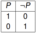
I ( ¬ P ) = { 0 if I ( P ) = 1 1 if I ( P ) = 0 I(\lnot P)=\begin{cases}0&\text{if}~I(P)=1\\1&\text{if}~I(P)=0\end{cases} I(¬P)={01if I(P)=1if I(P)=0
The corresponding truth table is:
6.3 Tautology
A tautology is a formula which is true under all interpretations.
⊤ : = ( p 1 ∨ ¬ p 1 ) \top:=(p_1\lor\lnot p_1) ⊤:=(p1∨¬p1)
6.4 Contradiction
A contradiction is a formula which is false under all interpretations.
⊥ : = ( p 1 ∧ ¬ p 1 ) \bot:=(p_1\land\lnot p_1) ⊥:=(p1∧¬p1)
6.5 Semantic consequence
Suppose Γ \Gamma Γ is a finite set of formulas and P P P is a formula. Then P P P follows from Γ \Gamma Γ (or is a semantic consequence of Γ \Gamma Γ) if the following implication holds for every interpretation I I I: if I ( Q ) = 1 for all Q ∈ Γ , then I ( P ) = 1 \text{if}~I(Q)=1~\text{for all}~Q\in\Gamma,~\text{then}~I(P)=1 if I(Q)=1 for all Q∈Γ, then I(P)=1This is denoted by Γ ⊨ P \Gamma\vDash P Γ⊨P
P 不一定在集合 Γ \Gamma Γ 内
The following conditions are equivalent:
- { P } ⊨ Q \{P\}\vDash Q {P}⊨Q
- ( P → Q ) (P\rightarrow Q) (P→Q) is a tautology
- ( P ∧ ¬ Q ) (P\land\lnot Q) (P∧¬Q) is a contradiction
6.5 Logical equivalence
Two formulas P P P and Q Q Q are called equivalent if they have the same truth value under every possible interpretation. In other words, P P P and Q Q Q are equivalent if I ( P ) = I ( Q ) I(P) = I(Q) I(P)=I(Q) for every interpretation I I I. This is denoted by P ≡ Q P\equiv Q P≡Q
Laws for equivalences
- Associative laws: ( P ∨ ( Q ∨ R ) ) ≡ ( ( P ∨ Q ) ∨ R ) (P\lor(Q\lor R))\equiv((P\lor Q)\lor R) (P∨(Q∨R))≡((P∨Q)∨R)
- Commutative laws: ( P ∨ Q ) ≡ ( Q ∨ P ) (P\lor Q)\equiv(Q\lor P) (P∨Q)≡(Q∨P)
- Identity laws: ( P ∨ ⊤ ) ≡ P (P\lor\top)\equiv P (P∨⊤)≡P
- Distributive laws: ( P ∧ ( Q ∨ R ) ) ≡ ( ( P ∧ Q ) ∨ ( P ∧ R ) ) (P\land(Q\lor R))\equiv((P\land Q)\lor(P\land R)) (P∧(Q∨R))≡((P∧Q)∨(P∧R))
- Complement laws: P ∨ ¬ P ≡ ⊤ P\lor\lnot P\equiv\top P∨¬P≡⊤
- De Morgan’s laws: ¬ ( P ∨ Q ) ≡ ( ¬ P ∧ ¬ Q ) \lnot(P\lor Q)\equiv(\lnot P\land\lnot Q) ¬(P∨Q)≡(¬P∧¬Q)
The relation ≡ \equiv ≡ is an equivalence relation on P P P
7. Predicate Logic
Limitations of Propositional Logic
Propositional logic is good for dealing with statements built from basic propositions using and, or, not, if … But more complex statements cannot be expressed naturally in propositional logic.
So we need to extend propositional logic. Numerous extensions have been developed, among them:
Modal Logic: Adds elements to reason about necessityTemporal Logic: Adds elements to reason about time.Predicate Logic: Adds elements to reason about properties of objects
Quantifiers
- ∀ \forall ∀ : for all, Universal quantification
- ∃ \exists ∃ : there exists an, Existential quantification
e,g,
Every student is younger than some instructor.
this statement can be written symbolically using predicates, variables, and quantifiers:
∀ x ( S t u d e n t ( x ) → ∃ y ( Y o u n g e r ( x , y ) ∧ I n s t r u c t o r ( y ) ) ) \forall x(Student(x)\rightarrow\exists y(Younger(x,y)\land Instructor(y))) ∀x(Student(x)→∃y(Younger(x,y)∧Instructor(y)))
This is a typical formula in predicate logic
Predicate logic has two additional features:
Equality: allows to express that individuals are equal or notfunction symbols: allows to express functional dependencies between individuals
Function symbols can often be “simulated” by predicates, so they are not really necessary. But function symbols lead to more natural descriptions
7.1 The Language of Predicate Logic
Predicate logic allows us to express statements about
objects- their
properties and relationsto each other
Some terminologies :
Domain: a non-empty set of objectsConstants: concrete objects in the domainFunctions: takes objects in the domain as arguments and returns an object of the domainPredicates: takes objects in the domain as arguments and returns true or false. They describe properties of objects or relationships between objectsVariables: placeholders for concrete objects in the domainQuantifiers: for how many objects in the domain is the statement true
7.2 Syntax of predicate logic
Signatures
A signature defines the “vocabulary” relative to which formulae can be expressed
A signature is a set consisting of :
- predicate symbols, each with an associated arity
- function symbols, each with an associated arity
- constant symbols
8. Combinatorics
Special Case for sums and products
∑
i
∈
∅
f
(
i
)
=
0
\sum\limits_{i\in\empty}f(i)=0
i∈∅∑f(i)=0
∏
i
∈
∅
f
(
i
)
=
1
\prod\limits_{i\in\empty}f(i)=1
i∈∅∏f(i)=1
permutations
A n m = n ! ( n − k ) ! A^m_n=\frac{n!}{(n-k)!} Anm=(n−k)!n!
subsets
C n m = n ! ( n − k ) ! k ! C^m_n=\frac{n!}{(n-k)!k!} Cnm=(n−k)!k!n!
The quantity which gives the number of size-k subsets of a set of size n, is called a binomial coefficient
It is writen an
(
k
n
)
(^n_k)
(kn) and pronounced “n choose k”
8.1 Discrete Probability
The sample space Ω \Omega Ω is the set of all possible outcomes. Every element x x x of Ω \Omega Ω has a probability P r ( x ) ∈ [ 0 , 1 ] Pr(x)\in[0,1] Pr(x)∈[0,1] ∑ x ∈ Ω P r ( x ) = 1 \sum\limits_{x\in\Omega}Pr(x)=1 x∈Ω∑Pr(x)=1
Events
An event is a subset X ⊆ Ω X\subseteq\Omega X⊆Ω. The probability of the event is given by P r ( X ) = ∑ x ∈ X P r ( x ) Pr(X)=\sum_{x\in X}Pr(x) Pr(X)=∑x∈XPr(x)
P
r
(
∅
)
=
0
Pr(\empty)=0
Pr(∅)=0
P
r
(
Ω
)
=
1
Pr(\Omega)=1
Pr(Ω)=1
P r ( X ∪ Y ) = P r ( X ) + P r ( Y ) − P r ( X ∩ Y ) Pr(X\cup Y)=Pr(X)+Pr(Y)-Pr(X\cap Y) Pr(X∪Y)=Pr(X)+Pr(Y)−Pr(X∩Y)
8.2 Conditional Probability
P r ( X ∣ Y ) = P r ( X ∩ Y ) P r ( Y ) Pr(X|Y)=\frac{Pr(X\cap Y)}{Pr(Y)} Pr(X∣Y)=Pr(Y)Pr(X∩Y)
8.3 Independence
Suppose that P r ( X ) ≠ 0 Pr(X)\ne0 Pr(X)=0 and P r ( Y ) ≠ 0 Pr(Y)\ne0 Pr(Y)=0. We say that events X X X and Y Y Y, are independent if P r ( X ∩ Y ) = P r ( X ) P r ( Y ) Pr(X\cap Y)=Pr(X)Pr(Y) Pr(X∩Y)=Pr(X)Pr(Y)
that is, P r ( X ∣ Y ) = P r ( X ) Pr(X|Y)=Pr(X) Pr(X∣Y)=Pr(X)
8.4 A random variable
A random variable is a function with domain Ω \Omega Ω
8.5 Expectation
The expected value of a random variable f is defined as follows E [ f ] = ∑ x ∈ Ω f ( x ) P r ( x ) E[f]=\sum_{x\in\Omega}f(x)Pr(x) E[f]=x∈Ω∑f(x)Pr(x)
This is sometimes called the expectation of f f f or the mean of f f f. It is the value that you expect to get if you pick x x x randomly from Ω \Omega Ω and then compute f ( x ) f(x) f(x)
If you repeatedly pick x x x randomly from Ω \Omega Ω and compute f ( x ) f(x) f(x) and you compute the average of the f ( x ) f(x) f(x) values, this tends towards E [ f ] E[f] E[f].
Linearity of expectation
If f and g are two random variables, then E [ f + g ] = E [ f ] + E [ g ] E[f+g]=E[f]+E[g] E[f+g]=E[f]+E[g]
If g ( x ) = c f ( x ) g(x)=cf(x) g(x)=cf(x), then E [ g ] = c E [ f ] E[g]=cE[f] E[g]=cE[f]
But E [ f × g ] = E [ f ] × E [ g ] E[f\times g]=E[f]\times E[g] E[f×g]=E[f]×E[g] is not always true


 1109
1109


 被折叠的 条评论
为什么被折叠?
被折叠的 条评论
为什么被折叠?
 到【灌水乐园】发言


