Time Series Diffusion Method: A Denoising Diffusion Probabilistic Model for Vibration Signal Genera

Time Series Diffusion Method: A Denoising Diffusion Probabilistic Model for Vibration Signal Genera

Abstract

Diffusion models have demonstrated robust data generation capabilities in various research fields.
In this paper, a Time Series Diffusion Method (TSDM) is proposed for vibration signal generation, leveraging the foundational principles of diffusion models.

扩散模型已经在各个研究领域展示了强大的数据生成能力。利用扩散模型的基本原理，提出了一种用于振动信号生成的时间序列扩散方法(TSDM)。

The TSDM improves the U-net architecture to effectively segment and extract features from one-dimensional time series data. It operates based on forward diffusion and reverse denoising processes for time-series generation.

TSDM改进了U-net体系结构，可以有效地从一维时间序列数据中分割和提取特征。它基于时间序列生成的正向扩散和反向去噪过程。

Experimental validation is conducted using single-frequency, multi-frequency datasets, and bearing fault datasets. The results show that TSDM can accurately generate the single-frequency and multi-frequency features in the time series and retain the basic frequency features for the diffusion generation results of the bearing fault series.

使用单频、多频数据集和轴承故障数据集进行实验验证。结果表明，TSDM可以准确地生成时间序列中的单频和多频特征，并保留轴承故障序列扩散生成结果的基本频率特征。

Finally, TSDM is applied to the small sample fault diagnosis of three public bearing fault datasets, and the results show that the accuracy of small sample fault diagnosis of the three datasets is improved by 57.5%, 22.7% and 21.4% at most, respectively.

最后，将TSDM应用于3个公共轴承故障数据集的小样本故障诊断，结果表明，3个数据集的小样本故障诊断准确率最高分别提高了57.5%、22.7%和21.4%。

1.Introduction

背景
Diffusion model is a new generation model that has developed rapidly in the field of Artificial Intelligence Generated Content (AIGC) in recent years[1] . It is called the new State of The Art (SOTA) model in the deep generation model[2]. The concept of diffusion model was proposed by Sohl-Dickstein et al.[3] in 2015, it was inspired by the diffusion movement in thermodynamics. For example, we drop a drop of red dye into a glass of pure water, the diffusion of dye molecules in the water is random. After a long enough time, the red dye will be evenly dispersed in the water, becoming a glass of red dye solution, which is the diffusion process as shown in Fig. 1. If we record the diffusion trajectory of each red dye molecule and move it in the opposite direction, we can eventually get a drop of red dye and a cup of pure water again.

扩散模型是近年来在人工智能生成内容(AIGC)领域迅速发展起来的新一代模型[1]。在深度生成模型[2]中被称为new State of the Art (SOTA)模型。扩散模型的概念由Sohl-Dickstein等人提出[3]2015年，灵感来自热力学中的扩散运动。例如，我们滴一滴红色染料到一杯纯净水中，染料分子在水中的扩散是随机的。经过足够长的时间后，红色染料会均匀地分散在水中，成为一杯红色染料溶液，其扩散过程如图1所示。如果我们记录下每个红色染料分子的扩散轨迹，并将其向相反的方向移动，我们最终可以得到一滴红色染料和一杯纯净水。

This reverse movementprocess is the generative process（生成过程）. Suppose we process another cup of the same concentration of dye solution according to the recorded trajectory information. In that case, we will also theoretically get a drop of dye and a cup of pure water. Suppose we record the diffusion trajectory information（记录扩散轨迹） of different concentrations of dye solutions. In that case, we can eventually achieve the reverse production of different concentrations of dye solutions into dye and pure water. This process of diffusion and reversal can be regarded as a diffusion model.

这种反向运动过程就是生成过程。假设我们根据记录的轨迹信息处理了另一杯相同浓度的染液。在这种情况下，理论上我们也会得到一滴染料和一杯纯水。假设我们记录不同浓度染液的扩散轨迹信息。在这种情况下在这种情况下，我们最终可以实现将不同浓度的染料溶液反向生成染料和纯水。染料溶液反向生成染料和纯水。这种扩散和反向生成的过程可被视为扩散模型。

Diffusion model could only generate low-pixel images at first, but it began to be widely promoted in 2020.

diffusion的发展

扩散模型最初只能生成低像素图像，但在2020年开始被广泛推广。

（1）Berkeley et al.[4] proposed Denoising Diffusion Probabilistic Models (DDPM(去噪扩散概率模型)) for image generation, which surpassed Generative Adversarial Nets (GANs) in the authenticity, diversity and even aesthetic of the generated images, and the training process was more stable.
In DDPM, U-net[5] is introduced to train and predict noise, significantly improving the diffusion model’s diffusion generation ability. Since then, DDPM has demonstrated powerful capabilities in many fields[6] . In Computational Vision (CV), Saharia et al.[7] proposed a general conditional diffusion model for image-to-image translation, superior to GANs in four tasks: colourization, inpainting, uncropping, and JPEG decompression（着色、上画、解裁剪和JPEG解压缩四个任务上优于GAN）.

Berkeley等[4]提出了用于图像生成的去噪扩散概率模型(Denoising Diffusion Probabilistic Models, DDPM)，该模型在生成图像的真实性、多样性甚至审美性方面都超过了生成对抗网络(Generative Adversarial Nets,GANs)，并且训练过程更加稳定。在DDPM中，引入U-net[5]对噪声进行训练和预测，显著提高了扩散模型的扩散生成能力。从那时起，DDPM在许多领域展示了强大的能力[6]。在计算视(Computational Vision,CV)中，撒哈拉等人[7]提出了一种用于图像到图像转换的通用条件扩散模型，该模型在着色、上画、解裁剪和JPEG解压缩四个任务上优于gan。Batzolis等[8]通过理论分析证明了基于分数的扩散模型的优越性，并引入了多速扩散框架对模型进行了改进，为研究多速扩散提供了基准。

（2）Yang et al.[9]proposed neural video coding algorithms presented various architectures that achieve
state-of-the-art performance in compressing high-resolution videos and delved into their trade-offs and variations.

提出的神经视频编码算法提出了各种架构，这些架构在压缩高分辨率视频方面实现了最先进的性能，并深入研究了它们的权衡和变化。

（3）Rombach et al. [10] proposed a novel model that combines a diffusion model with highly effective pretrained autoencoders（高效预训练自编码器）. This integration enabled the training of diffusion models even with constrained computational resources while maintaining their quality and flexibility. In contrast to prior research, training diffusion models on such a representation allowed for achieving a nearly optimal balance between complexity reduction and detail preservation, significantly enhancing visual fidelity

Rombach等人[10]提出了一种将扩散模型与高效预训练自编码器相结合的新模型。这种集成使扩散模型的训练即使在有限的计算资源下也能保持其质量和灵活性。与之前的研究相比，在这种表示上训练扩散模型可以在复杂性降低和细节保留之间实现近乎最佳的平衡，显著提高视觉保真度

（4）Yang et al. [11] proposed an autoregressive, end-to-end optimized video diffusion model, drawing inspiration from recent advancements in neural video compression. This model sequentially produces forthcoming frames by refining a deterministic next-frame prediction by integrating a stochastic residual generated via an inverse diffusion process.

Yang等[11]从神经视频压缩的最新进展中汲取灵感，提出了一种自回归的端到端优化视频扩散模型。该模型通过对逆扩散过程产生的随机残差进行积分，对确定性下一帧预测进行细化，进而产生下一帧。

Furthermore, owing to its formidable generative capabilities, diffusion models have made substantial strides in various domains, including Natural Language Processing (NLP) [12-14], Waveform Signal Processing [15,16], Molecular Graph Modeling [17-20], and Adversarial Purification [21-23]

此外，由于其强大的生成能力，扩散模型在各个领域取得了长足的进步，包括自然语言处理(NLP)[1214]、波形信号处理[15,16]、分子图建模[17-20]和对抗性净化[21-23]。

In the field of rotational machinery fault diagnosis based on Machine Learning (ML), research often necessitates extensive training data to build ML models[24-26]. However, collecting a substantial volume of training data in practical engineering settings can be excessively time-consuming, expensive, or even infeasible[27]. Consequently, the challenge of fault diagnosis with small samples has garnered widespread attention among researchers. The primary approach to address this issue is dataset expansion[28].
故障检测领域缺数据问题

在基于机器学习（ML）的旋转机械故障诊断领域，研究通常需要大量的训练数据来构建ML模型[24-26]。然而，在实际工程环境中收集大量训练数据可能非常耗时、昂贵，甚至是不可行的[27]。因此，小样本故障诊断的挑战引起了研究人员的广泛关注。解决这个问题的主要方法是数据集扩展[28]。

Presently, dataset expansion primarily relies on techniques such as interpolation to generate additional data（插值） from the small samples, forming an adequate training set for ML models[29,30]. Data generation methods encompass various data augmentation techniques [31,32], generative adversarial networks (GANs) [33-35], and more.

目前，数据集扩展主要依靠插值等技术从小样本中生成额外的数据，形成ML模型的适当训练集[29,30]。数据生成方法包括各种数据增强技术[31,32]，生成对抗网络(gan)[33-35]等。

（1）Li et al. [36] proposed a data augmentation method based on diverse signal processing techniques, and the results indicated that with a sufficiently large number of generated samples, the diagnostic performance of fault diagnosis models improved.

Li等[36]提出了一种基于多种信号处理技术的数据增强方法，结果表明，当生成的样本数量足够大时，故障诊断模型的诊断性能得到了提高。

（2） Ma et al. [37] proposed an enhanced version of traditional GANs known as Sparse Constraint GAN (SCGAN). SCGAN exhibited good convergence properties and effectively improved diagnosis accuracy.

Ma等人[37]提出了传统GAN的增强版本，称为稀疏约束GAN (SCGAN)。SCGAN具有良好的收敛性能，有效提高了诊断准确率。

（3）Wang et al. [38] presented an approach based on Sub-Pixel Convolutional Neural Networks
(ESPCN), which could produce high-quality synthetic data and significantly improve the accuracy of rotational machinery fault diagnosis. However, applying GANs requires training two adversarial networks, which is difficult and costly.

Wang等[38]提出了一种基于亚像素卷积神经网络(Sub-Pixel Convolutional Neural Networks,ESPCN)的方法，可以产生高质量的合成数据，显著提高旋转机械故障诊断的准确性。然而，应用gan需要训练两个对抗网络，这是困难和昂贵的。

本文研究TSDM

This paper proposes a Time Series Diffusion Method (TSDM) for vibration signal generation, leveraging the robust data generation capabilities of DDPM.
The TSDM enhances the U-net architecture to enable segmentation and feature extraction of onedimensional time series data, and it is founded on forward diffusion and reverse denoising processes for time series generation.
Through diffusion-based generation experiments on single-frequency, multi-frequency, and bearing datasets, the accuracy and effectiveness of the TSDM generation results are validated. Finally, the TSDM is applied to small sample fault diagnosis on three public bearing fault datasets, demonstrating that its application significantly improves the accuracy of small sample fault diagnosis.

利用DDPM的鲁棒数据生成能力，提出了一种用于振动信号生成的时间序列扩散方法(TSDM)。
TSDM对U-net结构进行了改进，实现了一维时间序列数据的分割和特征提取，并建立在时间序列生成的前向扩散和反向去噪过程的基础上。 通过单频、多频和轴承数据集的扩散生成实验，验证了TSDM生成结果的准确性和有效性。
最后，将该方法应用于三个公共轴承故障数据集的小样本故障诊断，结果表明，该方法的应用显著提高了小样本故障诊断的准确率。

2. Basic Theory

Denoising Diffusion Probabilistic Models (DDPM)[4] are based on the diffusion model, including forward diffusion, reverse denoising processes and model optimization. The specific principle is as follows.

去噪扩散概率模型(Diffusion probistic Models, DDPM)[4]基于扩散模型，包括正向扩散、反向去噪和模型优化。
具体原理如下:

2.1 Forward Diffusion Process

The forward diffusion process is the process of gradually adding Gaussian noise to the data until it ultimately becomes random noisy data.
For the raw data that will undergo T-step diffusion, the result obtained from each diffusion step is obtained by adding Gaussian noise to the previous step data , described in Eq.(1).

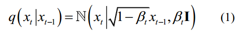
正向扩散过程是在数据中逐渐加入高斯噪声，直至最终成为随机噪声数据的过程。对于将进行t步扩散的原始数据x0~q(x0)，通过对前一步数据xt-1加入高斯噪声得到每个扩散步骤的结果xt，如式(1)所示。

where is the variance of Gaussian distribution noise at each step. As step increases, the variance needs to be taken larger, but it needs to satisfy as follow:

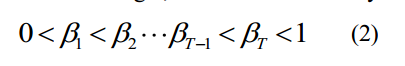
其中1 T T=为高斯分布噪声在每一步的方差。随着步长t的增加，需要取较大的方差t，但需要满足如下条件:

If the diffusion step is large enough, the result data will lose its original information and become random noise data. The entire diffusion process is a Markov chain from to ：

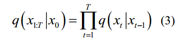
如果扩散步长T足够大，则结果数据将失去其原始信息，成为随机噪声数据。整个扩散过程是一条从t=1到t= t的马尔可夫链:

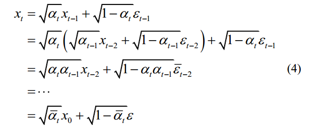
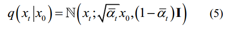
:The diffusion process is often fixed by using a pre-defined variance schedule. An essential feature of the forward diffusion process is that it can directly sample xt at any step t based on the original data . If and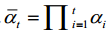 are defined, then through the reparamazation, the diffusion process can be expressed as follows:

扩散过程通常通过使用预定义的变化时间表来固定。正向扩散过程的一个本质特征是可以直接基于原始数据x0在任意步t处对xt进行采样:xt~q(xt
| x0)。若定义1 t t= -和1 t ti i= =，则通过重拟，扩散过程可表示为

:

where 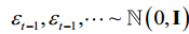, and merges two Gaussians. can be called the noise schedule. is a hyperparameter set with a noise schedule. Then, the diffusion process can be expressed as follows:

其中，(1，，~ 0，(1))和(2)t(1)合并两个高斯函数。1 T T T=可称为噪声表。1 t t II=变速=是一个带噪声调度的超参数集。则扩散过程可表示为:

The above is the entire process of the forward diffusion progress. can be seen as a linear combination of the original data and random noise , where and are the combination coefficients. Adjusting parameter to change the results generated by diffusion is more direct than variance . For example, if is set to a value close to 0, the resulting data is closer to Gaussian noise; If is set to a value close to T, the resulting data is closer to the original data.

以上就是正向扩散过程的整个过程。Xt可以看作是原始数据x0和随机噪声的线性组合，其中t和1
t−是组合系数。调整参数T来改变扩散产生的结果比方差T更直接。例如，如果T设置为接近0的值，则结果数据更接近高斯噪声;如果将T设置为接近T的值，则结果数据更接近原始数据。

2.2 Reverse Denoising Process

The reverse denoising process is based on the true distribution of each step, gradually denoising from a random noise , and ultimately generating the target data. Use a neural network to learn the distribution of the entire training sample and obtain the parameterized distribution 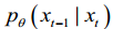of the neural network. The reverse process is also defined as a Markov chain.p can be expressed as follows:

反向去噪过程是根据每一步的真实分布q(xt-1 | xt)，从一个随机噪声xt ~ 0，(I)逐渐去噪，最终生成目标数据。使用神经网络学习整个训练样本的分布q(xt-1 | xt)，得到神经网络的参数化分布p x x (t t−1 |)。相反的过程也被定义为马尔可夫链。P可以表示为:

where is a parameter of the neural network. a random Gaussian noise, is a parameterized Gaussian distribution that requires the training network to calculate the mean and variance

.其中，为神经网络的参数。p x x (T T) = (;0,I)是随机高斯噪声，p x x (T T -1)是参数化高斯分布，需要训练网络计算平均值(x T T，)和方差(x T T，)。

3.3 Model Optimization

In the reverse denoising process, the true distribution is approximated to the parameterized distribution
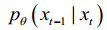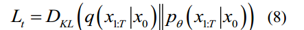
of the neural network. The optimization goal of TSDM is to make as close to as possible. This can be translatedinto finding the minimum KL divergence[2] oftwo joint distributions for two distributions, which can be defined as the loss function :

在反向去噪过程中，真实分布 q(xt-1 | xt) 被近似为 参数化分布 p x x  ( t t -1 | )的参数化分布。TSDM 的优化目标 TSDM 的优化目标是使 p x x  ( t t -1 | ) | ) 尽可能接近 q(xt-1 | xt)。这可以转化为寻找两个分布的两个联合分布的最小 KL 发散[2]、 可定义为损失函数 Lt ：

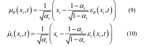
The mean of and can be written as follow:

p x x的平均值(tt−1 |)和q(xt-1 | xt)可以写成如下:

The loss function of step can be written as:

步骤t-1的损失函数Lt-1可以写成:

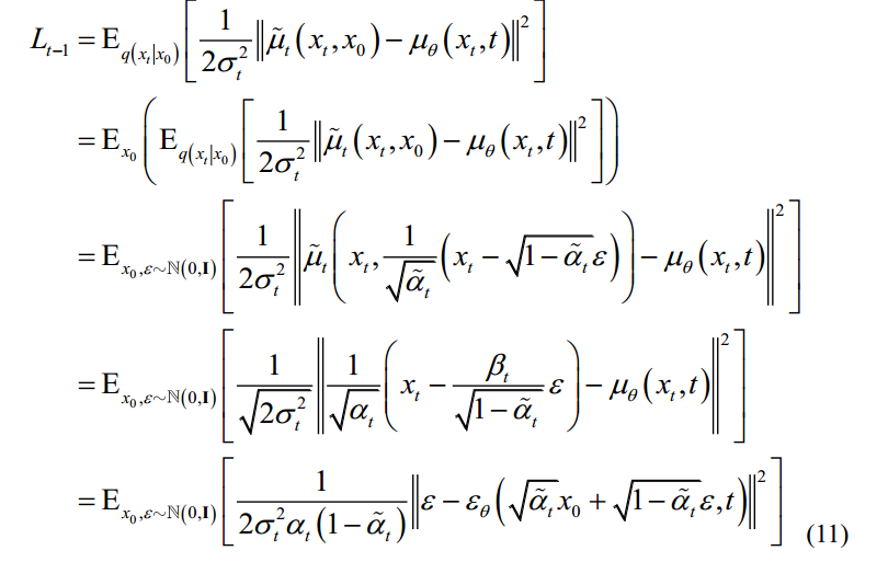
where represents the obtained by adding noise to original data . is a fitting function based on neural networks, which means that the model has switched from the original predicted mean to the predicted noise .

式中，xt表示对原始数据x0加入噪声ε得到的xt (x0，ε)。εθ是一个基于神经网络的拟合函数，这意味着模型已经从原来的预测均值切换到预测噪声ε。

By removing the weight coefficients of the target loss function, a further simplified result can be obtained as follows[4]:

通过去除目标损失函数的权系数，可以得到进一步简化的结果如下[4]:

3 Time Series Diffusion Method

3.1 U-net architecture

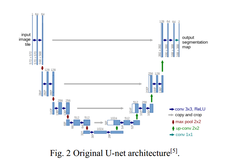
U-net [5] is widely used in the field of semantic segmentation in image processing and machine vision. The original U-net architecture is shown in Fig. 2. In the TSDM proposed in this study, TimeEbedding, ResBlock and AttnBlock are introduced to improve U-net to realize the noise prediction mechanism. The U-net architecture in this study is asymmetric, as shown in Fig. 3.


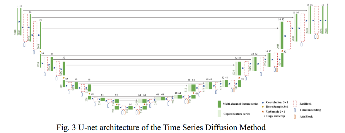
In the down-sampling process, the feature series enters the DownSample block after four convolutions and two ResBlock. The DownSample block can save practicalinformation and reduce the dimension of features to avoid overfitting. In the middle sampling stage, the feature series enters the UpSample block after four convolutions and two ResBlock. The AttnBlock is added to each ResBlock to retain features. In the upsampling stage, the feature series enters the UpSample block after six convolutions and three ResBlock. Each feature series in the down-sampling process is copied and concatenated in the up-sampling process to achieve the retention of the same dimensional features, which is conducive to network optimization.The AttnBlock is applied in the 3rd ResBlock to achieve better learning offeatures and increase the global modelling ability of the network. The TimeEbedding is fused with feature series in each ResBlock for model prediction and can implement U-net model sharing.

3.2 TSDM architecture

Based on the forward diffusion and reverse denoising processes in the Basic Theory, combined with the U-net network and the loss function used to optimize the network, the architecture of TSDM is shown in Fig. 4 to Fig. 6. The training diagram of TSDM is demonstrated in Fig. 4.

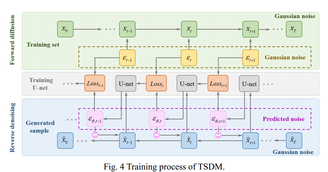
The training of TSDM is essentially the training of the U-net neural network in the model. In the forward diffusion process, Gaussian noise
t is added to the training sample xt at each step t, and finally, xT is generated through T-step diffusion, which is almost Gaussian noise. In the reverse denoising process, for each tx, it is input into the U-net neural network to predict the denoising noise ,t . The predicted noise
,t  and the Gaussian noise t added in the forward diffusion process (training process) are substituted into the loss function formula to update the U-net model and realize the optimization of the model. The U-net neural network optimization process in TSDM is shown in Fig. 5.

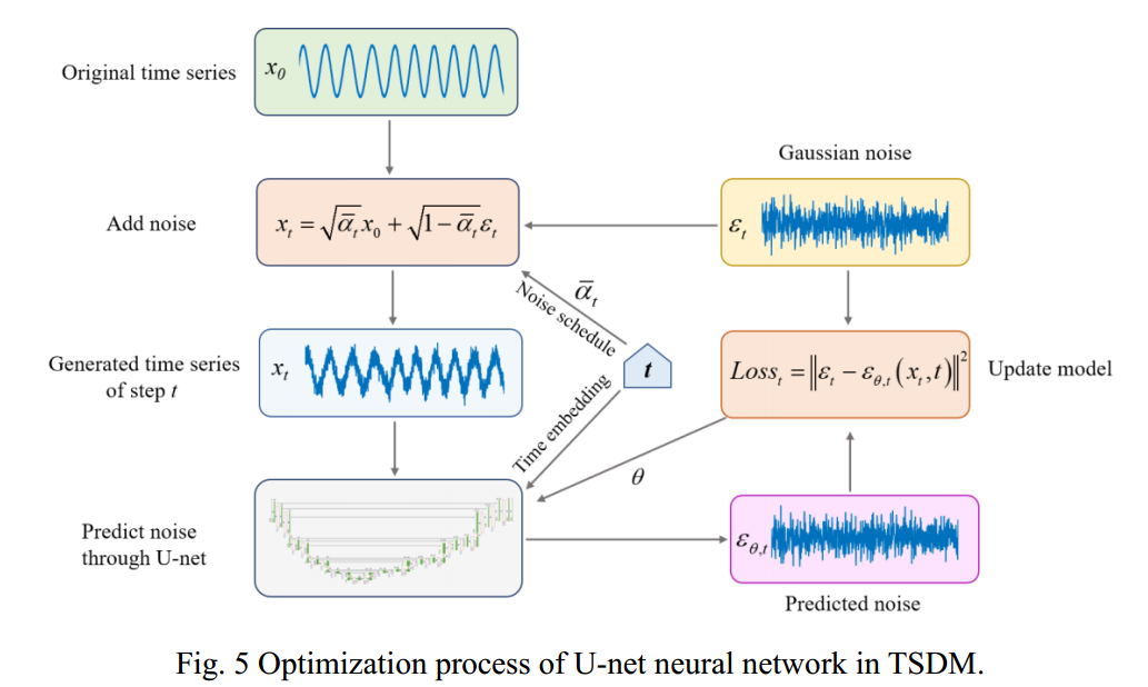
In the optimization process, optimization is actually carried out through a random time step t, rather than through each time step t, which will significantly improve the efficiency of optimization training. The noise schedule is generated according to the time step t, and the generated time series with added noise is trained through u-net. TimeEbedding is used to record the time step t during the training process. The loss function between the noise ,t predicted by u-net and the added Gaussian noise tis calculated, and the neural network parameter is updated. Next, take another random time step t for the next cycle until the end of the optimization process. At the end of the U-net optimization process, TSDM has also completed training and can generate time series by diffusion. The diffusion generation process of TSDM is shown in Fig. 6.

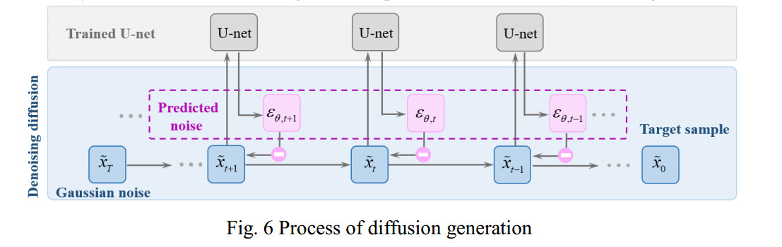
The diffusion generation process is to denoise the Gaussian noise sample Txlayer by layer. The final generated target sample is determined by the noise ,t denoised in each step t, and the noise ,t is predicted by the trained U-net. Finally, the target time series0x is generated, it has the characteristics of the training set and contains new random features, which makes the generated results expand the training set samples

4. Experimental Results

本节以人工构建的时间序列数据集和已发表的轴承故障数据集为例，通过比较生成序列与原始序列的特征相似度，检验本文提出的时间序列扩散方法的有效性。使用的数据集包括单频时间序列、多频时间序列和XJTU[43]轴承故障数据集。

4.1 Single-frequency Time Series

A single-frequency time series dataset is constructed by trigonometric function. The construction method is as follows:

利用三角函数构造单频时间序列数据集。施工方法如下:

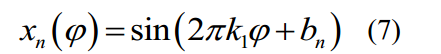
式中，k1为预设频率;Bn是0 ~ 2π之间的随机数，用于时间序列之间的相位差，避免数据之间的过拟合。

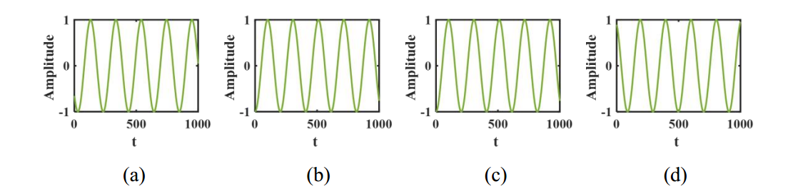
A single-frequency time series dataset of 10Hz is built according to Eq.(7), and the dataset size is [200,2048], which contains 200 time series with a length of 2048. Partial time series in the single-frequency dataset are shown in Fig. 7.

During the forward diffusion and training process, the batch size is set to 10, and the TSDM is trained over 200 epochs to realize denoising generation. The number of noise diffusion and denoising layers T is set to 3000. Based on the trained model, 40 target time
series are generated, partial results are shown in Fig. 8, and the corresponding frequency spectrum is shown in Fig. 9.

在正向扩散和训练过程中，将批大小设置为10，对TSDM进行200次以上的训练，以实现去噪的生成。噪声扩散和去噪层数T设置为3000。基于训练好的模型，生成了40个目标时间序列，部分结果如图8所示，对应的频谱如图9所示。

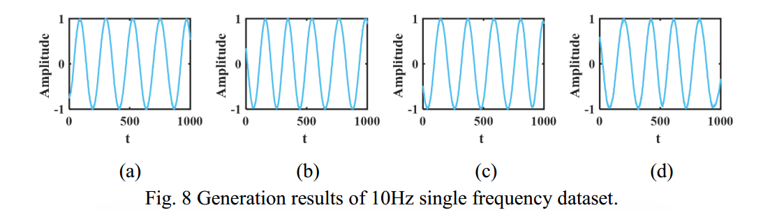
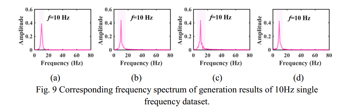
在10Hz单频数据集的扩散生成结果中，如图8所示，扩散生成的时间序列呈现三角函数的标准形式，且周期一致。图9为生成结果对应的频谱，可以看出扩散生成后10Hz的特征频率得到了很好的保存，反映了生成结果的准确性。

但各频谱主峰的带宽存在差异，这是生成结果随机性的体现。这意味着TSDM生成的结果在保持主要特征的同时具有一定的随机性。这也表明TSDM可以生成多样化的目标时间序列，而不是简单地复制训练样本。

将生成的40个时间序列的频谱进行汇总，绘制出如图10所示的箱形图。从箱形图中可以看出，生成的时间序列的频率分量的峰值主要在特征频率附近。
但是，与其他频率位置相比，峰值的幅度波动较大，可以看出平均频谱峰值的带宽明显比单个样本的带宽宽。所得频谱峰值的幅度和带宽的不确定性反映了TSDM的创造性。

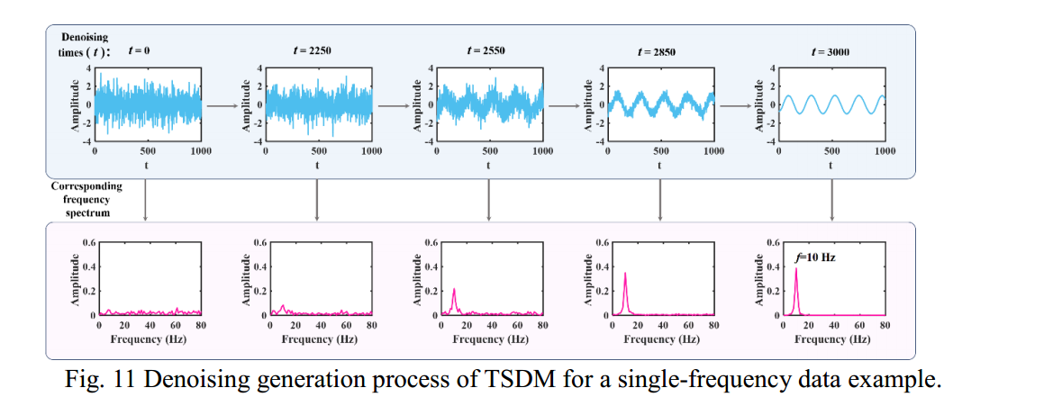
Fig. 10 Box plot of generation results of 10Hz single frequency dataset Taking the generated result in Fig. 8(a) as an example, draw the process of gradually denoising it from random noise to generating a single-frequency trigonometric function, as shown in Fig. 11. From the denoising generation process, it can be seen that with the increase of denoising times t, the random noise first gradually forms the contour of the target sequence. For example, when t=2550, a rough outline appears, and when t=2850, the shape is so apparent that the periodicity of the target series can be seen. It can also be seen from the corresponding frequency spectrum that with the increase of denoising times, the corresponding peak of the characteristic frequency of the target series gradually appears and increases. In the U-net architecture of TSDM, because U-net is a shared parameter, the role of TimeEbedding is to let the model form the general outline of the series and learn the critical feature information when it is close to generating the target series. This dramatically improves the efficiency of TSDM generation.

图 10 10Hz 单频数据集生成结果的方框图 以图 8（a）中的生成结果为例，绘制从随机噪声逐步去噪到生成单频三角函数的过程、 如图 11
所示。从去噪生成过程可以看出，随着去噪次数 t 随着去噪次数 t 的增加，随机噪声首先逐渐形成目标序列的轮廓。目标序列的轮廓。例如，当 t=2550 时，会出现一个粗略的轮廓，而当 t=2850 时、 形状非常明显，可以看到目标序列的周期性。还可以从相应的频谱也可以看出，随着去噪次数的增加 目标序列特征频率的相应峰值逐渐出现并增大。出现并增大。在 TSDM 的 U-net 结构中，由于U-net 是一个共享参数，因此 TimeEbed 的作用是将目标序列的特征频 在 TSDM 的 U-net 架构中，由于 U-net是一个共享参数，TimeEbedding 的作用是让模型形成序列的总体轮廓，并在学习关键特征信息时并在接近生成目标序列时学习关键特征信息。时学习关键特征信息。这极大地提高了 TSDM 生成的效率。

4.2 Multi-frequency Time Series

利用三角函数构造了多频时间序列数据集。施工方法如下:

式中，k1, k2，…km为预设频率;B1n, b2n，…，bmn为0 ~ 2π之间的随机数，用于相同频率的时间序列之间的相位差，避免过拟合。

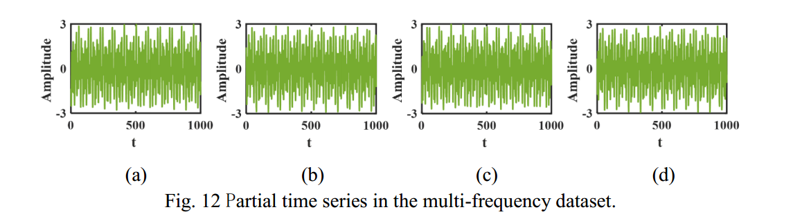
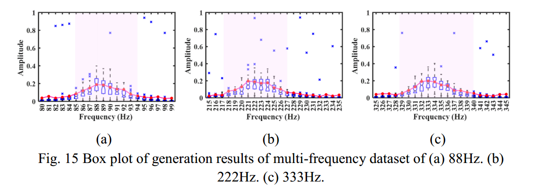
在本研究中，根据式(8)将三个不同频率的时间序列组合成一个多频时间序列，其中k1=88 k2=222 k3=333。数据集大小为[200,2048]，包含200个时间序列，长度为2048。多频数据集中的部分时间序列如图12所示。

在正向扩散和训练过程中，将批大小设置为10，对TSDM进行200次以上的训练，以实现去噪的生成。噪声扩散和去噪层数T设置为3000。基于训练好的模型，生成了40个目标时间序列，部分结果如图13所示，对应的频谱如图14所示。

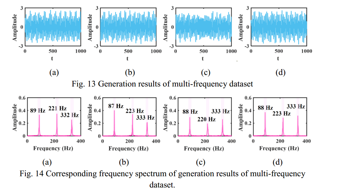
在多频率数据集的扩散生成结果中，可以从图 13 中看出，扩散生成的时间序列显示出标准节拍特征。13 中可以看出，扩散生成的时间序列显示了多频序列中经常出现的标准节拍特征。多频率序列中经常出现的标准节拍特征，且周期性一致。图 14 显示了 图 14 显示了生成结果的相应频谱。图 14 显示了相应的频谱生成结果。这反映了生成结果的准确性。由于频率较高 某些生成结果的频率误差不超过 2%，这是可以接受的。在多频率生成结果的频谱中，生成结果的随机性比单频率生成结果更明显。在多频生成结果频谱中，生成结果的随机性比单频生成结果更为明显。三个特征频率的带宽 三个特征频率的带宽和振幅在生成结果之间是不同的。这也意味着 TSDM 的生成结果在保留主要特征的同时，具有一定的随机性。这也说明 TSDM 生成的结果在保留主要特征的同时，还具有一定的随机性。这也说明 TSDM 可以生成多样化的目标时间序列，而不是简单地复制训练结果。在多频率时间序列训练后，TSDM 可以生成多样化的目标时间序列，而不是简单地复制训练样本训练。
将生成的40个时间序列的频谱进行汇总，绘制出如图15所示的箱形图。从箱形图中可以看出，生成的时间序列的频率分量的峰值主要在特征频率附近。与其他频率位置相比，峰值的幅度波动较大，可以看出平均频谱峰值的带宽明显宽于单个样本的带宽。所得频谱峰值的幅度和带宽的不确定性反映了TSDM的创造性。此外，可以看出，在多频生成结果中，离群值的数量远远多于单频生成结果，这也说明TSDM对于具有更多特征的目标时间序列更具创造性。

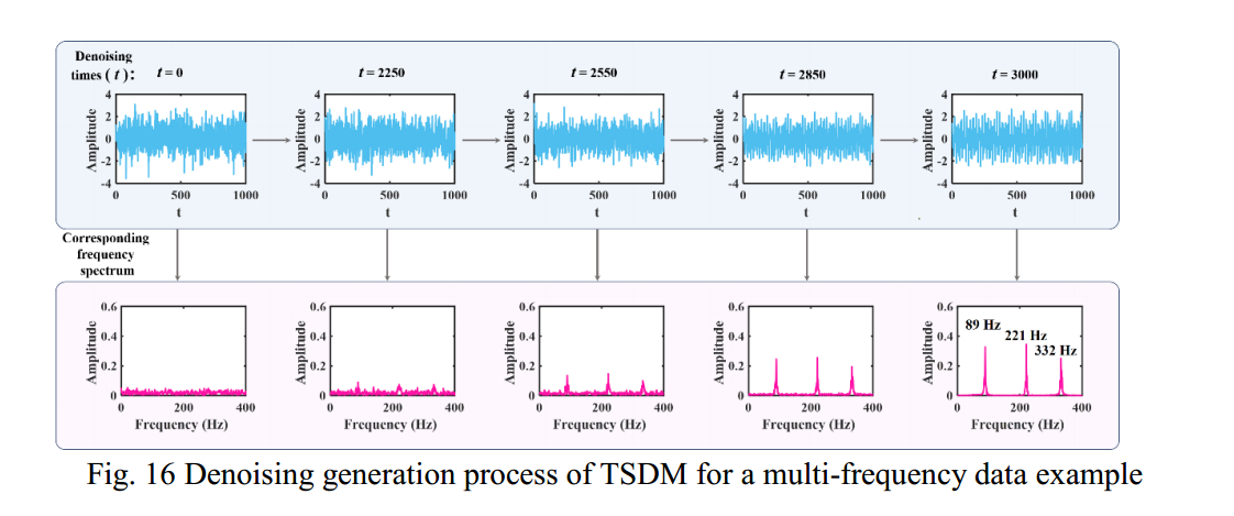
以图13(a)生成的结果为例，画出从随机噪声逐步去噪到生成单频三角函数的过程，如图16所示。从去噪的产生过程可以看出，随着去噪次数t的增加，随机噪声首先逐渐形成目标序列的轮廓。从对应的频谱可以看出，随着去噪次数的增加，目标序列特征频率对应的峰值逐渐出现并增大。由于时间序列中有三个频率分量，所以在t=3000之前不能清楚地看到序列的拍频现象。

4.3 Bearing Fault Data

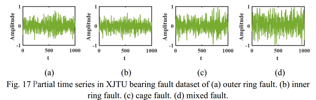
在4.1节和4.2节中，通过人工构建单频和多频时间序列数据集，证明了TSDM对正则序列出色的扩散生成能力。为了测试TSDM生成实际振动信号的能力，也决定了其是否可以在实践中应用，本节选择一个公开的轴承故障数据集来训练TSDM并进行扩散生成。所选的XJTU轴承故障数据集包括外圈故障、内圈故障、保持架故障和混合故障。数据集大小为[200,2048]，其中包含每个故障的200个时间序列，长度为2048。XJTU数据集的部分时间序列如图17所示。

During the forward diffusion and training process, the batch size is set to 10, and the TSDM is trained over 200 epochs to realize denoising generation. The number of noise diffusion and denoising layers T is set to 3000. Based on the trained model, 40 target time series of each fault are generated, and a partial of the results is shown in Fig. 18. Because the speed corresponding to the same fault data in the bearing fault dataset is different, it also leads to the fault characteristic frequency corresponding to the same fault may be different. To reflect the retention of the generated results on the fault characteristics, the frequency spectrum of the same fault in the dataset is summarized and averaged, and drawn in the same figure as the frequency spectrum of the generated results, as shown in Fig. 19.

在前向扩散和训练过程中，批量大小设为 10，TSDM 经过 200 个历时训练，以实现去噪生成。噪声扩散和去噪层数 T 设为3000。根据训练好的模型，生成每个故障的 40 个目标时间序列，部分结果如图 18 所示。由于轴承故障数据集中同一故障数据对应的转速不同，也导致同一故障对应的故障特征频率可能不同。为反映生成结果对故障特征的保留，对数据集中同一故障的频谱进行汇总和平均，并绘制成与生成结果频谱相同的图，如图19 所示。

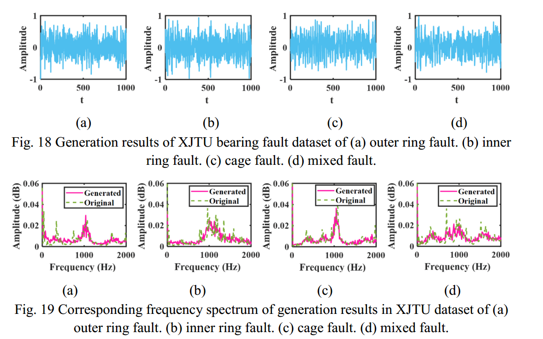
在XJTU轴承故障数据集的扩散生成结果中，如图所示。17 .扩散生成的时间序列不能直接观测到故障特征，这与单频和多频时间序列数据集的结果不同。这也意味着保存和生成轴承故障数据集的特征是一项更加困难的任务。在图19中，蓝色虚线表示训练集中200个数据的平均频谱，红色实线表示单个生成结果的频谱。可以看出，平均频谱的谱线相对平滑，而生成的结果谱线明显有更多的频率成分。总体而言，生成结果的频谱与训练集的平均频谱趋势一致，两者具有较高的重合程度。这表明，TSDM可以生成与训练集具有相似特征的轴承故障时间序列。这也证明了TSDM可以生成简单的标准时间序列和实测数据，这将大大拓展TSDM的应用前景。

5. Application Instance

在第4节中，TSDM对单频时间序列、多频时间序列和轴承故障数据表现出出色的生成能力。在实际的基于深度学习的故障诊断中，由于缺乏训练样本，诊断的准确率会较低，称为小样本故障诊断。合理扩展小样本训练集将有效解决这一问题。在本节中，我们定义了一个小样本故障诊断案例，并通过 TSDM 对小样本数据集进行扩展，以提高故障诊断精度，如图 20 所示。

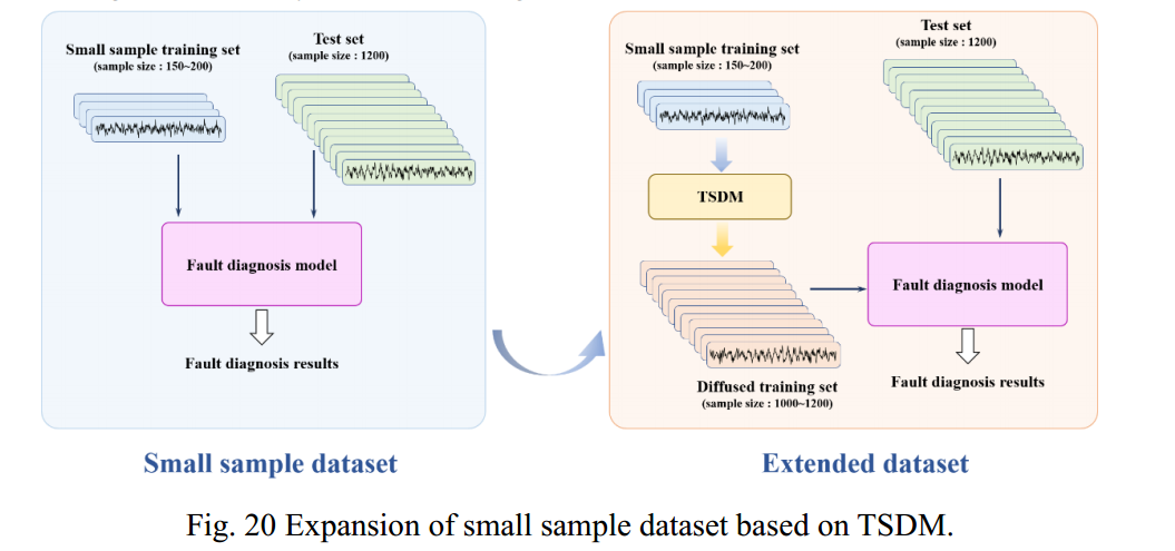
5.1 Small sample fault diagnosis under CWRU dataset[42]

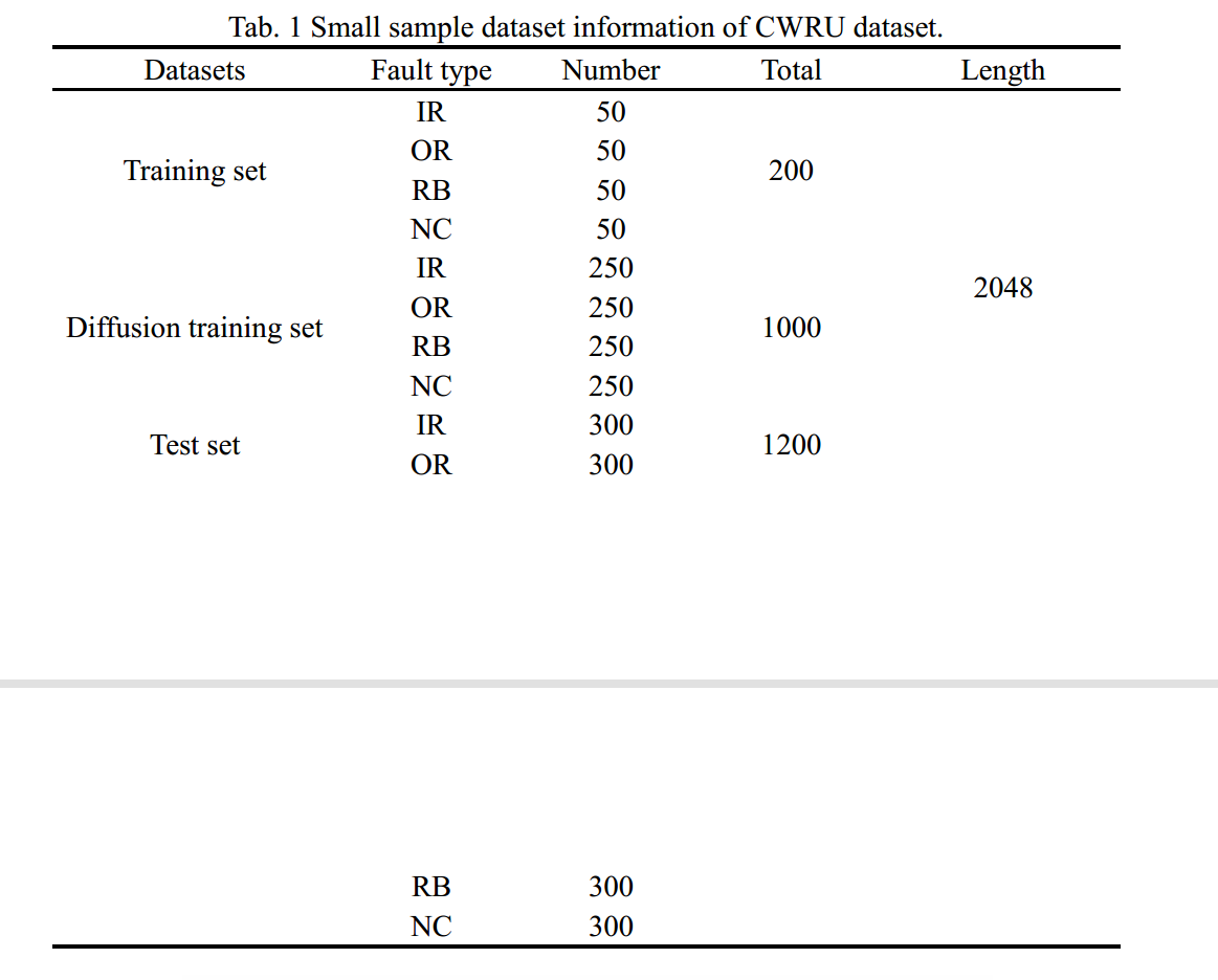
CWRU轴承故障数据集广泛应用于轴承故障诊断领域。研究人员通过电火花加工预制了内环故障(IR)、外环故障(OR)和滚球故障(RB)三种故障，以及无故障健康状态，并进行了无故障正常状态(NC)试验。对于IR、OR、RB和NC四种工况，每种工况随机抽取50个样本，共200个样本作为小样本训练集;每种工况选取300个样本，共选取1200个样本作为测试集。以小样本训练集作为扩散训练集，生成每个工况400个样本，共1200个样本。所用小样本数据集的基本信息如表1所示。

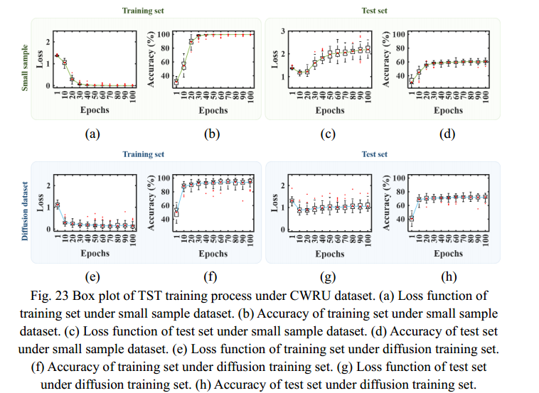
本研究选择CNN[39]、RNNLSTM[40]和TST[41]三种机器学习方法，对小样本数据集扩散前后的故障诊断结果进行比较。数据集大小设置为10，机器学习方法的训练次数分别超过100次，重复50次。使用扩散训练集前后，训练集和测试集在训练过程中的准确率和损失函数如图21 ~图23所示。



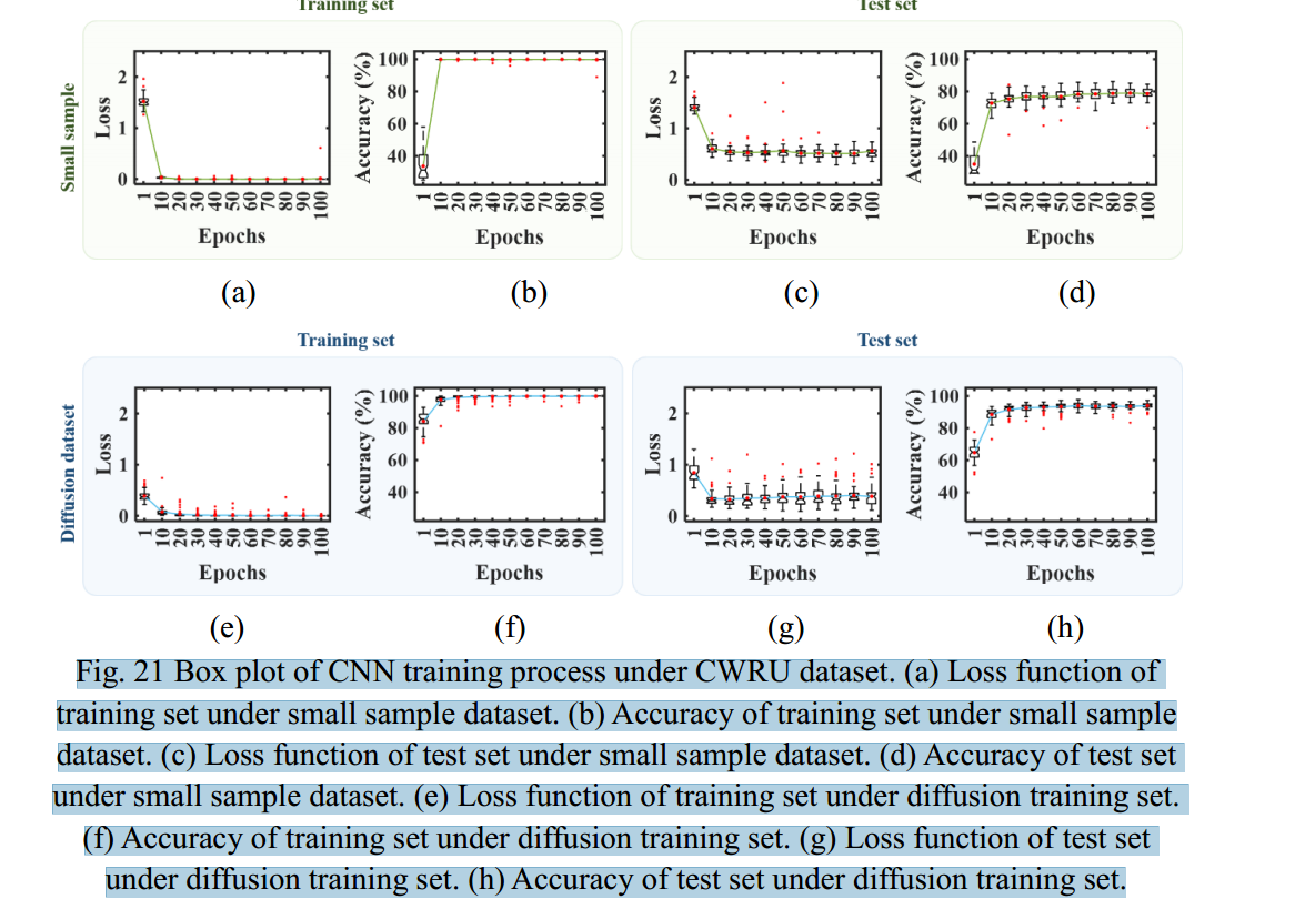
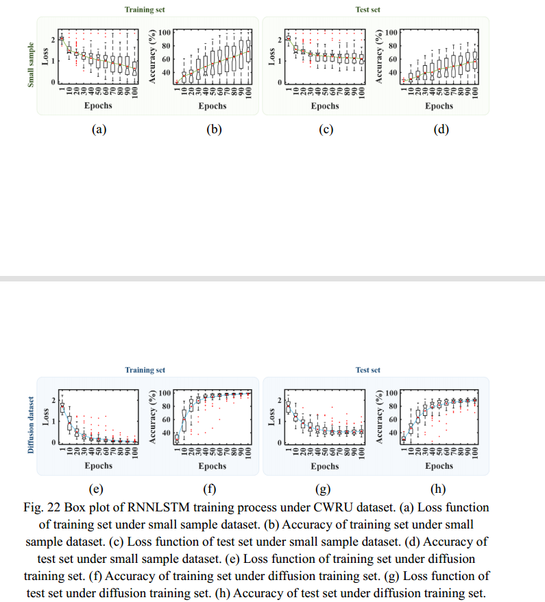
从图21中CNN的训练过程可以看出，与小样本数据集相比，基于扩散训练集的训练集的诊断准确率和损失函数更快到达平衡位置。测试集的诊断精度提高，损失函数显著降低。虽然数据集的扩散导致了基于扩散训练集的训练过程中异常值的增加，但CNN的整体诊断结果得到了积极的改善。从图22中RNNLSTM的训练过程可以看出，基于小样本数据集的训练结果是严重离散的，这体现在箱形图中，箱形太长，特别是在图22(a)、(b)和(d)中。同时，小样本训练集导致RNNLSTM在epoch=100之前没有收敛。使用扩散数据集后，这些问题得到了改善。从图中可以看出。22(e)、(f)、(g)、(h)，训练过程中的损失函数减小，诊断准确率显著提高。同时，训练过程呈现出良好的收敛趋势。
从图23中TST的训练过程可以看出，在基于小样本数据集的训练中，TST的结果主要存在测试集损失函数增大和诊断准确率不高的问题，如图23©和(d)所示。使用扩散训练集后，这两个问题得到了改善，图23(g)中损失函数逐渐减小，图23(g)中准确率略有提高。23 (h)。此外，使用扩散训练集后的训练集的损失函数和准确率比小样本数据集收敛得更快。

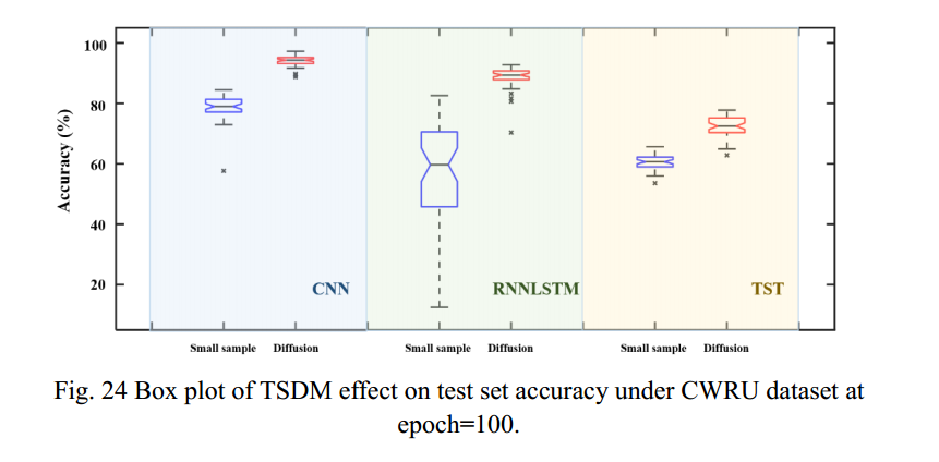
对epoch=100时测试集的准确率进行汇总，以反映TSDM的贡献，箱线图如图24所示，汇总表如表2所示。由图24可以看出，当将CNN、LSTM和TST应用于小样本数据集的训练和故障诊断时，将TSDM应用于小样本数据集的扩散生成处理后，诊断结果有明显改善。改进幅度在小样本数据集上分别为19.5%、57.6%和19.2%，如表2所示。

6. Conclusions

本文提出了一种基于扩散概率去噪模型的时间序列去噪方法。在TSDM中，对U-net进行了改进，使其适用于一维时间序列的分割和特征提取，并应用于TSDM的噪声预测。在单频、多频和轴承故障数据集上测试了该方法的有效性，并将其应用于小样本故障诊断。结论如下:(1)利用TSDM生成单频和多频人工构造的三角函数数据集。结果表明:生成的三角函数序列的周期性与原始序列一致，多频数据集生成的序列存在与原始序列相似的拍频现象。从生成的频谱可以看出，生成的时间序列很好地保留了原序列的频率特性。
(2)对公共轴承故障数据集进行弥散和TSDM生成。将生成序列的频谱与原始序列的平均频谱进行比较，结果表明，生成的时间序列频谱与原始序列的平均频谱高度拟合，证明了TSDM在扩散生成时能够保留实际振动信号的频率特性。这也意味着TSDM可以应用于故障诊断。
(3)基于CWRU、XJTU和HIT三个公开的轴承故障诊断数据集，定义了一个小样本故障诊断案例。利用TSDM生成小样本训练集，对数据集进行扩展。结果表明，当使用CNN、LSTM和TST对三种数据集进行小样本故障诊断时，TSDM生成的扩散数据集可以有效提高小样本故障诊断的准确率，最大提高了57%。
本文的研究结果表明，所提出的 TSDM 模型具有生成时间序列的强大能力。生成时间序列的能力。今后的工作重点是优化 TSDM 模型，提高其对小样本数据集的故障诊断准确性。提高其对小样本数据集的故障诊断准确性。本文中使用 TSDM 本文中使用 TSDM 进行的小样本故障诊断还不够全面，可与其他生成方法进行比较，研究其优越性。与其他生成方法进行比较，研究 TSDM 在处理小样本故障诊断方面的优越性。