改善深层神经网络-week2编程题（Optimization Methods）

1. Optimization Methods

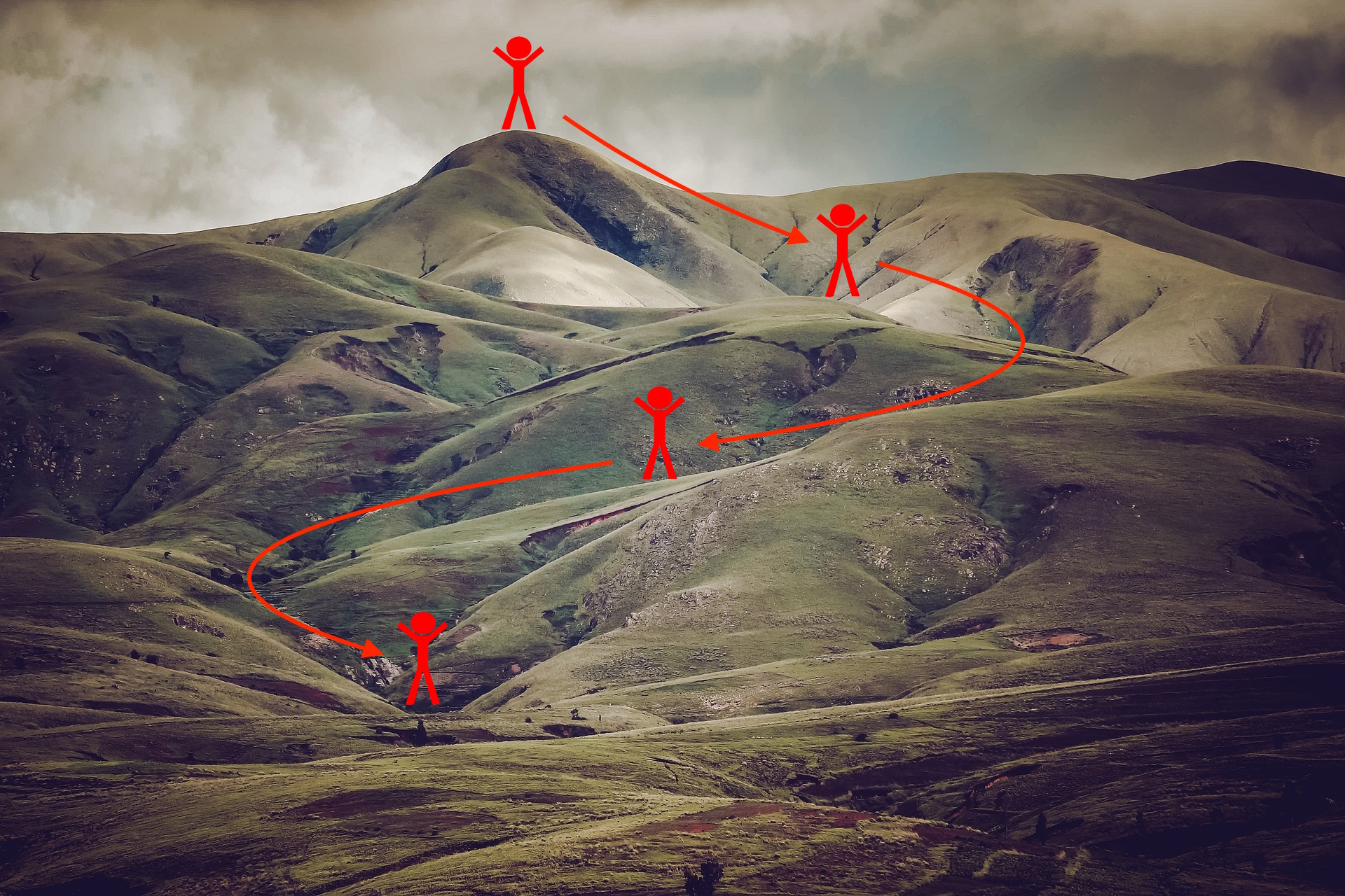
Gradient descent goes "downhill" on a cost function \(J\). Think of it as trying to do this:

**Figure 1** : **Minimizing the cost is like finding the lowest point in a hilly landscape**
At each step of the training, you update your parameters following a certain direction to try to get to the lowest possible point.

Notations: As usual, \(\frac{\partial J}{\partial a}=\) da for any variable a.

To get started, run the following code to import the libraries you will need.

import numpy as np
import matplotlib.pyplot as plt
import scipy.io
import math
import sklearn
import sklearn.datasets

from opt_utils import load_params_and_grads, initialize_parameters, forward_propagation, backward_propagation
from opt_utils import compute_cost, predict, predict_dec, plot_decision_boundary, load_dataset
from testCases import *

%matplotlib inline
plt.rcParams['figure.figsize'] = (7.0, 4.0) # set default size of plots
plt.rcParams['image.interpolation'] = 'nearest'
plt.rcParams['image.cmap'] = 'gray'

1.1 - Gradient Descent

A simple optimization method in machine learning is gradient descent (GD). When you take gradient steps with respect to all \(m\) examples on each step, it is also called Batch Gradient Descent.

Warm-up exercise: Implement the gradient descent update rule. The gradient descent rule is, for \(l = 1, ..., L\):

\[W^{[l]} = W^{[l]} - \alpha \text{ } dW^{[l]} \tag{1} \]

\[b^{[l]} = b^{[l]} - \alpha \text{ } db^{[l]} \tag{2} \]

where L is the number of layers and \(\alpha\) is the learning rate. All parameters should be stored in the parameters dictionary. Note that the iterator l starts at 0 in the for loop while the first parameters are \(W^{[1]}\) and \(b^{[1]}\). You need to shift l to l+1 when coding.

# GRADED FUNCTION: update_parameters_with_gd

def update_parameters_with_gd(parameters, grads, learning_rate):
    """
    Update parameters using one step of gradient descent
    
    Arguments:
    parameters -- python dictionary containing your parameters to be updated:
                    parameters['W' + str(l)] = Wl
                    parameters['b' + str(l)] = bl
    grads -- python dictionary containing your gradients to update each parameters:
                    grads['dW' + str(l)] = dWl
                    grads['db' + str(l)] = dbl
    learning_rate -- the learning rate, scalar.
    
    Returns:
    parameters -- python dictionary containing your updated parameters 
    """

    L = len(parameters) // 2 # number of layers in the neural networks

    # Update rule for each parameter
    for l in range(L):
        ### START CODE HERE ### (approx. 2 lines)    
        parameters['W' + str(l+1)] = parameters['W' + str(l+1)] - learning_rate*grads['dW' + str(l+1)]
        parameters['b' + str(l+1)] = parameters['b' + str(l+1)] - learning_rate*grads['db' + str(l+1)]     
        ### END CODE HERE ###
        
    return parameters

测试：

parameters, grads, learning_rate = update_parameters_with_gd_test_case()

parameters = update_parameters_with_gd(parameters, grads, learning_rate)
print("W1 = " + str(parameters["W1"]))
print("b1 = " + str(parameters["b1"]))
print("W2 = " + str(parameters["W2"]))
print("b2 = " + str(parameters["b2"]))

输出：
W1 = [[ 1.63535156 -0.62320365 -0.53718766]
[-1.07799357 0.85639907 -2.29470142]]
b1 = [[ 1.74604067]
[-0.75184921]]
W2 = [[ 0.32171798 -0.25467393 1.46902454]
[-2.05617317 -0.31554548 -0.3756023 ]
[ 1.1404819 -1.09976462 -0.1612551 ]]
b2 = [[-0.88020257]
[ 0.02561572]
[ 0.57539477]]

A variant of this is Stochastic Gradient Descent (SGD), which is equivalent to mini-batch gradient descent where each mini-batch has just 1 example. The update rule that you have just implemented does not change. What changes is that you would be computing gradients on just one training example at a time, rather than on the whole training set. The code examples below illustrate the difference between stochastic gradient descent and (batch) gradient descent.

• (Batch) Gradient Descent:

X = data_input
Y = labels
parameters = initialize_parameters(layers_dims)
for i in range(0, num_iterations):
    # Forward propagation
    a, caches = forward_propagation(X, parameters)
    # Compute cost.
    cost = compute_cost(a, Y)
    # Backward propagation.
    grads = backward_propagation(a, caches, parameters)
    # Update parameters.
    parameters = update_parameters(parameters, grads)

• Stochastic Gradient Descent:

X = data_input
Y = labels
parameters = initialize_parameters(layers_dims)
for i in range(0, num_iterations):
    for j in range(0, m):
        # Forward propagation
        a, caches = forward_propagation(X[:,j], parameters)
        # Compute cost
        cost = compute_cost(a, Y[:,j])
        # Backward propagation
        grads = backward_propagation(a, caches, parameters)
        # Update parameters.
        parameters = update_parameters(parameters, grads)

In Stochastic Gradient Descent, you use only 1 training example before updating the gradients. When the training set is large, SGD can be faster. But the parameters will "oscillate" toward the minimum rather than converge smoothly. Here is an illustration of this:

**Figure 1** : **SGD vs GD**
"+" denotes a minimum of the cost. SGD leads to many oscillations(振动) to reach convergence(收敛). But each step is a lot faster to compute for SGD than for GD, as it uses only one training example (vs. the whole batch for GD).

Note also that implementing SGD requires 3 for-loops in total:

1. Over the number of iterations
2. Over the \(m\) training examples
3. Over the layers (to update all parameters, from \((W^{[1]},b^{[1]})\) to \((W^{[L]},b^{[L]})\))

In practice, you'll often get faster results if you do not use neither the whole training set, nor only one training example, to perform each update. Mini-batch gradient descent uses an intermediate number of examples for each step. With mini-batch gradient descent, you loop over the mini-batches instead of looping over individual training examples.

**Figure 2** : **SGD vs Mini-Batch GD**
"+" denotes a minimum of the cost. Using mini-batches in your optimization algorithm often leads to faster optimization.

What you should remember:

• The difference between gradient descent, mini-batch gradient descent and stochastic gradient descent is the number of examples you use to perform one update step.
• You have to tune a learning rate hyperparameter \(\alpha\).
• With a well-turned mini-batch size, usually it outperforms either gradient descent or stochastic gradient descent (particularly when the training set is large).

1.2 - Mini-Batch Gradient descent

Let's learn how to build mini-batches from the training set (X, Y).

There are two steps:

• Shuffle(洗牌): Create a shuffled version of the training set (X, Y) as shown below. Each column of X and Y represents a training example. Note that the random shuffling is done synchronously(同步地) between X and Y. Such that after the shuffling the \(i^{th}\)