4.深度学习练习：Building your Deep Neural Network: Step by Step（强烈推荐）

本文节选自吴恩达老师《深度学习专项课程》编程作业，在此表示感谢。

课程链接：https://www.deeplearning.ai/deep-learning-specialization/

fter this assignment you will be able to:

• Use non-linear units like ReLU to improve your model
• Build a deeper neural network (with more than 1 hidden layer)
• Implement an easy-to-use neural network class

Notation:

• Superscriptdenotes a quantity associated with the  layer.
  • Example:  is the  layer activation.  and are the layer parameters.
• Superscript (i)denotes a quantity associated with the ??ℎith example.
  • Example: ?(?) is the training example.
• Lowerscript ?i denotes the ??ℎith entry of a vector.
  • Example: denotes the entry of the  layer's activations).

---

目录

1 - Packages

2 - Outline of the Assignment

3 - Initialization

3.1 - 2-layer Neural Network

3.2 - L-layer Neural Network¶

4 - Forward propagation module

4.1 - Linear Forward

4.2 - Linear-Activation Forward

4.3 L-Layer Model

5 - Cost function

6 - Backward propagation module

6.1 - Linear backward

6.2 - Linear-Activation backward

6.3 - L-Model Backward

6.4 - Update Parameters

7 - Conclusion

---

1 - Packages

Let's first import all the packages that you will need during this assignment.

• numpy is the main package for scientific computing with Python.
• matplotlib is a library to plot graphs in Python.
• dnn_utils provides some necessary functions for this notebook.
• testCases provides some test cases to assess the correctness of your functions
• np.random.seed(1) is used to keep all the random function calls consistent.

import numpy as np
import h5py
import matplotlib.pyplot as plt
from testCases_v2 import *
from dnn_utils_v2 import sigmoid, sigmoid_backward, relu, relu_backward

%matplotlib inline
plt.rcParams['figure.figsize'] = (5.0, 4.0) # set default size of plots
plt.rcParams['image.interpolation'] = 'nearest'
plt.rcParams['image.cmap'] = 'gray'

%load_ext autoreload
%autoreload 2

np.random.seed(1)

---

2 - Outline of the Assignment

To build your neural network, you will be implementing several "helper functions". These helper functions will be used in the next assignment to build a two-layer neural network and an L-layer neural network. Each small helper function you will implement will have detailed instructions that will walk you through the necessary steps. Here is an outline of this assignment, you will:

• Initialize the parameters for a two-layer network and for an L-layer neural network.
• Implement the forward propagation module (shown in purple in the figure below).
  • Complete the LINEAR part of a layer's forward propagation step (resulting in ).
  • We give you the ACTIVATION function (relu/sigmoid).
  • Combine the previous two steps into a new [LINEAR->ACTIVATION] forward function.
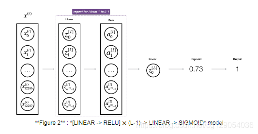
  • Stack the [LINEAR->RELU] forward function L-1 time (for layers 1 through L-1) and add a [LINEAR->SIGMOID] at the end (for the final layer L). This gives you a new L_model_forward function.
• Compute the loss.
• Implement the backward propagation module (denoted in red in the figure below).
  • Complete the LINEAR part of a layer's backward propagation step.
  • We give you the gradient of the ACTIVATE function (relu_backward/sigmoid_backward)
  • Combine the previous two steps into a new [LINEAR->ACTIVATION] backward function.
  • Stack [LINEAR->RELU] backward L-1 times and add [LINEAR->SIGMOID] backward in a new L_model_backward function
• Finally update the parameters.

Note that for every forward function, there is a corresponding backward function. That is why at every step of your forward module you will be storing some values in a cache. The cached values are useful for computing gradients. In the backpropagation module you will then use the cache to calculate the gradients. This assignment will show you exactly how to carry out each of these steps.

---

3 - Initialization

You will write two helper functions that will initialize the parameters for your model. The first function will be used to initialize parameters for a two layer model. The second one will generalize this initialization process to ?L layers.

3.1 - 2-layer Neural Network

Exercise: Create and initialize the parameters of the 2-layer neural network.

Instructions:

• The model's structure is: LINEAR -> RELU -> LINEAR -> SIGMOID.
• Use random initialization for the weight matrices. Use np.random.randn(shape)*0.01 with the correct shape.
• Use zero initialization for the biases. Use np.zeros(shape).

def initialize_parameters(n_x, n_h, n_y):
    """
    Argument:
    n_x -- size of the input layer
    n_h -- size of the hidden layer
    n_y -- size of the output layer
    
    Returns:
    parameters -- python dictionary containing your parameters:
                    W1 -- weight matrix of shape (n_h, n_x)
                    b1 -- bias vector of shape (n_h, 1)
                    W2 -- weight matrix of shape (n_y, n_h)
                    b2 -- bias vector of shape (n_y, 1)
    """
    
    np.random.seed(1)
    
    W1 = np.random.randn(n_h, n_x) * 0.01
    b1 = np.zeros((n_h, 1))
    W2 = np.random.randn(n_y, n_h) * 0.01
    b2 = np.zeros((n_y, 1))
    assert(W1.shape == (n_h, n_x))
    assert(b1.shape == (n_h, 1))
    assert(W2.shape == (n_y, n_h))
    assert(b2.shape == (n_y, 1))
    
    parameters = {"W1": W1,
                  "b1": b1,
                  "W2": W2,
                  "b2": b2}
    
    return parameters    

3.2 - L-layer Neural Network¶

Exercise: Implement initialization for an L-layer Neural Network.

Instructions:

• The model's structure is [LINEAR -> RELU] ×× (L-1) -> LINEAR -> SIGMOID. I.e., it has ?−1 layers using a ReLU activation function followed by an output layer with a sigmoid activation function.
• Use random initialization for the weight matrices. Use np.random.rand(shape) * 0.01.
• Use zeros initialization for the biases. Use np.zeros(shape).
• We will store , the number of units in different layers, in a variable layer_dims. For example, the layer_dims for the "Planar Data classification model" from last week would have been [2,4,1]: There were two inputs, one hidden layer with 4 hidden units, and an output layer with 1 output unit. Thus means W1's shape was (4,2), b1 was (4,1), W2 was (1,4) and b2 was (1,1). Now you will generalize this to L layers!
• Here is the implementation for L=1 (one layer neural network). It should inspire you to implement the general case (L-layer neural network).

    if L == 1:
        parameters["W" + str(L)] = np.random.randn(layer_dims[1], layer_dims[0]) * 0.01
        parameters["b" + str(L)] = np.zeros((layer_dims[1], 1))

def initialize_parameters_deep(layer_dims):
    """
    Arguments:
    layer_dims -- python array (list) containing the dimensions of each layer in our network
    
    Returns:
    parameters -- python dictionary containing your parameters "W1", "b1", ..., "WL", "bL":
                    Wl -- weight matrix of shape (layer_dims[l], layer_dims[l-1])
                    bl -- bias vector of shape (layer_dims[l], 1)
    """
    
    np.random.seed(3)
    parameters = {}
    L = len(layer_dims)            # number of layers in the network

    for l in range(1, L):
      
        parameters["W" + str(l)] = np.random.rand(layer_dims[l], layer_dims[l-1]) * 0.01
        parameters["b" + str(l)] = np.zeros((layer_dims[l], 1))
        
        assert(parameters['W' + str(l)].shape == (layer_dims[l], layer_dims[l-1]))
        assert(parameters['b' + str(l)].shape == (layer_dims[l], 1))

        
    return parameters

---

4 - Forward propagation module

4.1 - Linear Forward

Now that you have initialized your parameters, you will do the forward propagation module. You will start by implementing some basic functions that you will use later when implementing the model. You will complete three functions in this order:

• LINEAR
• LINEAR -> ACTIVATION where ACTIVATION will be either ReLU or Sigmoid.
• [LINEAR -> RELU] ×× (L-1) -> LINEAR -> SIGMOID (whole model)

The linear forward module (vectorized over all the examples) computes the following equations:

Exercise: Build the linear part of forward propagation.

def linear_forward(A, W, b):
    """
    Implement the linear part of a layer's forward propagation.

    Arguments:
    A -- activations from previous layer (or input data): (size of previous layer, number of examples)
    W -- weights matrix: numpy array of shape (size of current layer, size of previous layer)
    b -- bias vector, numpy array of shape (size of the current layer, 1)

    Returns:
    Z -- the input of the activation function, also called pre-activation parameter 
    cache -- a python dictionary containing "A", "W" and "b" ; stored for computing the backward pass efficiently
    """
    

    Z = np.dot(W, A) + b
    
    assert(Z.shape == (W.shape[0], A.shape[1]))
    cache = (A, W, b)
    
    return Z, cache

4.2 - Linear-Activation Forward

In this notebook, you will use two activation functions:sigmoid and tanh

Exercise: Implement the forward propagation of the LINEAR->ACTIVATION layer. Mathematical relation is:  where the activation "g" can be sigmoid() or relu(). Use linear_forward() and the correct activation function.

def linear_activation_forward(A_prev, W, b, activation):
    """
    Implement the forward propagation for the LINEAR->ACTIVATION layer

    Arguments:
    A_prev -- activations from previous layer (or input data): (size of previous layer, number of examples)
    W -- weights matrix: numpy array of shape (size of current layer, size of previous layer)
    b -- bias vector, numpy array of shape (size of the current layer, 1)
    activation -- the activation to be used in this layer, stored as a text string: "sigmoid" or "relu"

    Returns:
    A -- the output of the activation function, also called the post-activation value 
    cache -- a python dictionary containing "linear_cache" and "activation_cache";
             stored for computing the backward pass efficiently
    """
    
    if activation == "sigmoid":
        # Inputs: "A_prev, W, b". Outputs: "A, activation_cache".
        Z, linear_cache = linear_forward(A_prev, W, b)
        A, activation_cache = sigmoid(Z)
   
    
    elif activation == "relu":
        Z, linear_cache = linear_forward(A_prev, W, b)
        A, activation_cache = relu(Z)
    
    assert (A.shape == (W.shape[0], A_prev.shape[1]))
    cache = (linear_cache, activation_cache)

    return A, cache

4.3 L-Layer Model

For even more convenience when implementing the L-layer Neural Net, you will need a function that replicates the previous one (linear_activation_forward with RELU) L−1times, then follows that with one linear_activation_forward with SIGMOID.

Exercise: Implement the forward propagation of the above model.

Instruction: In the code below, the variable AL will denote  (This is sometimes also called Yhat, i.e., this is .)

Tips:

• Use the functions you had previously written
• Use a for loop to replicate [LINEAR->RELU] (L-1) times
• Don't forget to keep track of the caches in the "caches" list. To add a new value c to a list, you can use list.append(c).

def L_model_forward(X, parameters):
    """
    Implement forward propagation for the [LINEAR->RELU]*(L-1)->LINEAR->SIGMOID computation
    
    Arguments:
    X -- data, numpy array of shape (input size, number of examples)
    parameters -- output of initialize_parameters_deep()
    
    Returns:
    AL -- last post-activation value
    caches -- list of caches containing:
                every cache of linear_relu_forward() (there are L-1 of them, indexed from 0 to L-2)
                the cache of linear_sigmoid_forward() (there is one, indexed L-1)
    """

    caches = []
    A = X
    L = len(parameters) // 2                  # number of layers in the neural network
    
    # Implement [LINEAR -> RELU]*(L-1). Add "cache" to the "caches" list.
    for l in range(1, L):
        A_prev = A 
        A, cache = linear_activation_forward(A_prev, parameters["W" + str(l)], parameters["b" +str(l)], "relu")
        caches.append(cache)
    
    # Implement LINEAR -> SIGMOID. Add "cache" to the "caches" list.
   
    AL, cache = linear_activation_forward(A, parameters['W' + str(L)], parameters['b' + str(L)], "sigmoid")    # 注意这里是 A
    caches.append(cache)
    
    assert(AL.shape == (1,X.shape[1]))
            
    return AL, caches

---

5 - Cost function

Now you will implement forward and backward propagation. You need to compute the cost, because you want to check if your model is actually learning.

Exercise: Compute the cross-entropy cost ?, using the following formula:

def compute_cost(AL, Y):
    """
    Implement the cost function defined by equation (7).

    Arguments:
    AL -- probability vector corresponding to your label predictions, shape (1, number of examples)
    Y -- true "label" vector (for example: containing 0 if non-cat, 1 if cat), shape (1, number of examples)

    Returns:
    cost -- cross-entropy cost
    """
    
    m = Y.shape[1]

  
    cost = -1/m * np.sum(np.dot(Y, np.log(AL).T) + np.dot(1 - Y, np.log(1 - AL).T))
    
    cost = np.squeeze(cost)      # To make sure your cost's shape is what we expect (e.g. this turns [[17]] into 17).
    assert(cost.shape == ())
    
    return cost

---

6 - Backward propagation module

Just like with forward propagation, you will implement helper functions for backpropagation. Remember that back propagation is used to calculate the gradient of the loss function with respect to the parameters.

Now, similar to forward propagation, you are going to build the backward propagation in three steps:

• LINEAR backward
• LINEAR -> ACTIVATION backward where ACTIVATION computes the derivative of either the ReLU or sigmoid activation
• [LINEAR -> RELU] ×× (L-1) -> LINEAR -> SIGMOID backward (whole model)

6.1 - Linear backward

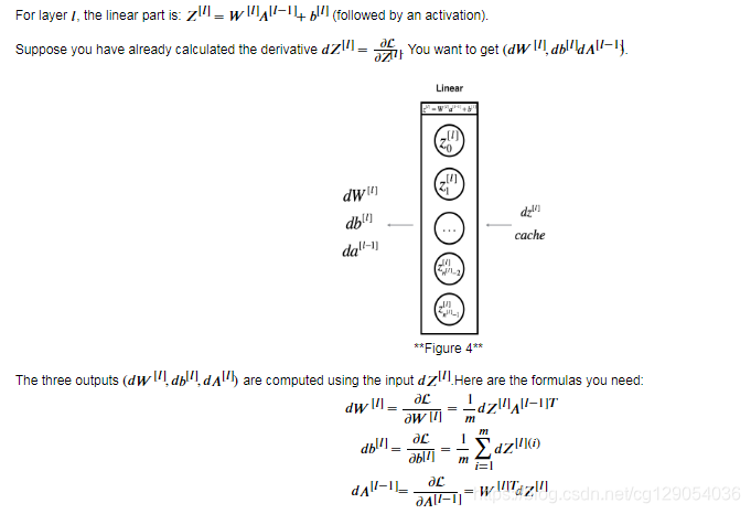
def linear_backward(dZ, cache):
    """
    Implement the linear portion of backward propagation for a single layer (layer l)

    Arguments:
    dZ -- Gradient of the cost with respect to the linear output (of current layer l)
    cache -- tuple of values (A_prev, W, b) coming from the forward propagation in the current layer

    Returns:
    dA_prev -- Gradient of the cost with respect to the activation (of the previous layer l-1), same shape as A_prev
    dW -- Gradient of the cost with respect to W (current layer l), same shape as W
    db -- Gradient of the cost with respect to b (current layer l), same shape as b
    """
    A_prev, W, b = cache
    m = A_prev.shape[1]
  
    dW = 1/m * np.dot(dZ, A_prev.T)
    db = 1/m * np.sum(dZ, axis=1, keepdims=True)
    dA_prev = np.dot(W.T, dZ)
    
    assert (dA_prev.shape == A_prev.shape)
    assert (dW.shape == W.shape)
    assert (db.shape == b.shape)
    
    return dA_prev, dW, db

6.2 - Linear-Activation backward

Next, you will create a function that merges the two helper functions: linear_backward and the backward step for the activation linear_activation_backward.

To help you implement linear_activation_backward, we provided two backward functions:

• sigmoid_backward: Implements the backward propagation for SIGMOID unit. You can call it as follows:

dZ = sigmoid_backward(dA, activation_cache)

• relu_backward: Implements the backward propagation for RELU unit. You can call it as follows:

dZ = relu_backward(dA, activation_cache)

If ?(.)g(.) is the activation function, sigmoid_backward and relu_backward compute

def linear_activation_backward(dA, cache, activation):
    """
    Implement the backward propagation for the LINEAR->ACTIVATION layer.
    
    Arguments:
    dA -- post-activation gradient for current layer l 
    cache -- tuple of values (linear_cache, activation_cache) we store for computing backward propagation efficiently
    activation -- the activation to be used in this layer, stored as a text string: "sigmoid" or "relu"
    
    Returns:
    dA_prev -- Gradient of the cost with respect to the activation (of the previous layer l-1), same shape as A_prev
    dW -- Gradient of the cost with respect to W (current layer l), same shape as W
    db -- Gradient of the cost with respect to b (current layer l), same shape as b
    """
    linear_cache, activation_cache = cache
    
    if activation == "relu":
       
        dZ = relu_backward(dA, activation_cache)
        dA_prev, dW, db = linear_backward(dZ, linear_cache)
        
    elif activation == "sigmoid":
     
        dZ = sigmoid_backward(dA, activation_cache)
        dA_prev, dW, db = linear_backward(dZ, linear_cache)

    
    return dA_prev, dW, db

6.3 - L-Model Backward

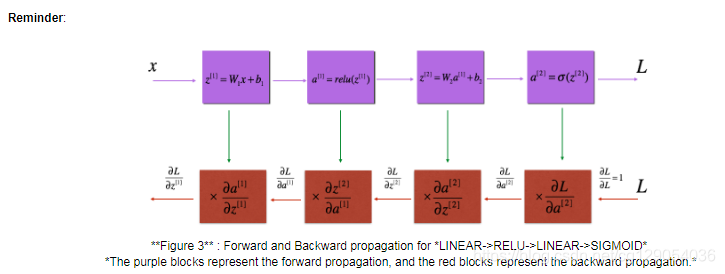
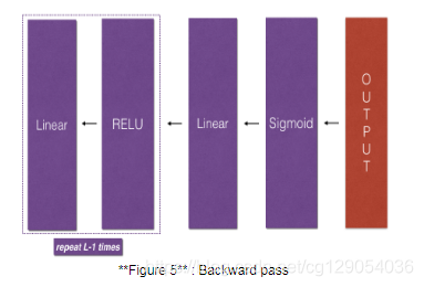
Now you will implement the backward function for the whole network. Recall that when you implemented the L_model_forward function, at each iteration, you stored a cache which contains (X,W,b, and z). In the back propagation module, you will use those variables to compute the gradients. Therefore, in the L_model_backward function, you will iterate through all the hidden layers backward, starting from layer L. On each step, you will use the cached values for layer ?l to backpropagate through layer l. Figure 5 below shows the backward pass.

** Initializing backpropagation**: To backpropagate through this network, we know that the output is, ?[?]=?(?[?])A[L]=σ(Z[L]). Your code thus needs to compute dAL =∂∂?[?]=∂L∂A[L]. To do so, use this formula (derived using calculus which you don't need in-depth knowledge of):

dAL = - (np.divide(Y, AL) - np.divide(1 - Y, 1 - AL)) # derivative of cost with respect to AL

You can then use this post-activation gradient dAL to keep going backward. As seen in Figure 5, you can now feed in dAL into the LINEAR->SIGMOID backward function you implemented (which will use the cached values stored by the L_model_forward function). After that, you will have to use a for loop to iterate through all the other layers using the LINEAR->RELU backward function. You should store each dA, dW, and db in the grads dictionary. To do so, use this formula :

?????["??"+???(?)]=??[?]

For example, for ?=3this would store ??[?]dW[l] in grads["dW3"].

Exercise: Implement backpropagation for the [LINEAR->RELU] ×× (L-1) -> LINEAR -> SIGMOID model.

def L_model_backward(AL, Y, caches):
    """
    Implement the backward propagation for the [LINEAR->RELU] * (L-1) -> LINEAR -> SIGMOID group
    
    Arguments:
    AL -- probability vector, output of the forward propagation (L_model_forward())
    Y -- true "label" vector (containing 0 if non-cat, 1 if cat)
    caches -- list of caches containing:
                every cache of linear_activation_forward() with "relu" (it's caches[l], for l in range(L-1) i.e l = 0...L-2)
                the cache of linear_activation_forward() with "sigmoid" (it's caches[L-1])
    
    Returns:
    grads -- A dictionary with the gradients
             grads["dA" + str(l)] = ...
             grads["dW" + str(l)] = ...
             grads["db" + str(l)] = ...
    """
    grads = {}
    L = len(caches) # the number of layers
    m = AL.shape[1]
    Y = Y.reshape(AL.shape) # after this line, Y is the same shape as AL

    # Initializing the backpropagation
 
    dAL = - (np.divide(Y, AL) - np.divide(1 - Y, 1 - AL))

    
    # Lth layer (SIGMOID -> LINEAR) gradients. Inputs: "AL, Y, caches". Outputs: "grads["dAL"], grads["dWL"], grads["dbL"]
 
    current_cache = caches[L-1]
    grads["dA" + str(L)], grads["dW" + str(L)], grads["db" + str(L)] = linear_activation_backward(dAL, current_cache, 'sigmoid')

    
    for l in reversed(range(L - 1)):
        # lth layer: (RELU -> LINEAR) gradients.
        # Inputs: "grads["dA" + str(l + 2)], caches". Outputs: "grads["dA" + str(l + 1)] , grads["dW" + str(l + 1)] , grads["db" + str(l + 1)] 
      
        current_cache = caches[l]
        dA_prev_temp, dW_temp, db_temp = linear_activation_backward(grads["dA" + str(l + 2)], caches[l], 'relu')
        grads["dA" + str(l + 1)] = dA_prev_temp
        grads["dW" + str(l + 1)] = dW_temp
        grads["db" + str(l + 1)] = db_temp
       

    return grads

6.4 - Update Parameters

def update_parameters(parameters, grads, learning_rate):
    """
    Update parameters using gradient descent
    
    Arguments:
    parameters -- python dictionary containing your parameters 
    grads -- python dictionary containing your gradients, output of L_model_backward
    
    Returns:
    parameters -- python dictionary containing your updated parameters 
                  parameters["W" + str(l)] = ... 
                  parameters["b" + str(l)] = ...
    """
    
    L = len(parameters) // 2 # number of layers in the neural network

    # Update rule for each parameter. Use a for loop.
    for l in range(L):
        parameters["W" + str(l+1)] = parameters["W" + str(l+1)] - learning_rate * grads["dW" + str(l + 1)]
        parameters["b" + str(l+1)] = parameters["b" + str(l+1)] - learning_rate * grads["db" + str(l + 1)]
        
    return parameters

---

7 - Conclusion

Congrats on implementing all the functions required for building a deep neural network!

We know it was a long assignment but going forward it will only get better. The next part of the assignment is easier.

In the next assignment you will put all these together to build two models:

• A two-layer neural network
• An L-layer neural network

You will in fact use these models to classify cat vs non-cat images!