R语言-2*2卡方检验与效应量

基础情境

一个任务有两个选项，多个不同年龄被试对此做出决策，获得两个年龄段选择两个选项的频次：

年龄	3-4	5-6
选项A	22	10
选项B	45	66

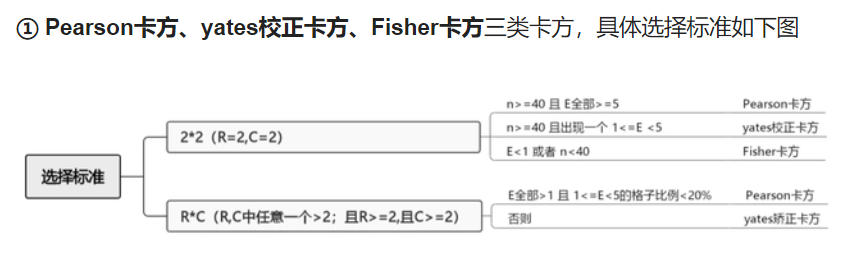
通过卡方检验对此进行分析，对应效应量指标为phi（φ）系数。

对于两个2×2的随机变量（x和y）:

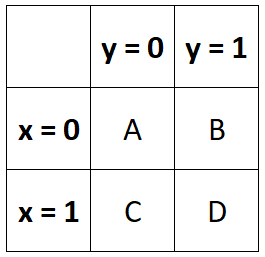
phi系数的计算公式: φ = (AD-BC) / √(A+B)(C+D)(A+C)(B+D)

R语言语句

方法一：prop.test()

该函数仅适用于有两个选项的情况，即一个被试只能做出是 vs. 否（或A vs. B）的回答。

#数据录入，先纵后横
data_chi = matrix(c(22,45,10,66),nrow = 2)

#统计检验
> prop.test(data_chi)

    2-sample test for equality of proportions with continuity correction

data:  data_chi
X-squared = 6.8455, df = 1, p-value = 0.008886
alternative hypothesis: two.sided
95 percent confidence interval:
 0.07721308 0.48697611
sample estimates:
   prop 1    prop 2 
0.6875000 0.4054054 

在统计检验过程中有一个校正的问题需要注意，对应参数correct，默认的分析报告了校正后的结果，若无需校正，定义correct = F。关闭校正后结果如下：

> prop.test(data_chi,correct = F)

    2-sample test for equality of proportions without continuity correction

data:  data_chi
X-squared = 7.938, df = 1, p-value = 0.004841
alternative hypothesis: two.sided
95 percent confidence interval:
 0.09734259 0.46684660
sample estimates:
   prop 1    prop 2 
0.6875000 0.4054054 

从p值可以发现，是否校正还是对显著性有一定的影响的。关于这个问题还是有一点争议，不过似乎更多的人倾向于使用校正后的结果。从网站讨论中找到了这样的建议（似乎主要对皮尔逊卡方）：

So, Yates showed that the use of Pearson's chi-squared has the implication of p–values which underestimate the true p–values based on the binomial distribution, but that you already know. Actually, statisticians tend to disagree about whether to use it: some statisticians argue that expected frequency lower that five should imply the use of that correction, while others use ten as that value, while others make the case that Yates' Correction should be used in every chi-squared tests with contingency tables 2 X 2.

ps. 上述网址中还包含另一种直接进行卡方检验的语句：

prop.test(x=c(226,181), n=c(365,335))

也就是直接定义x=0时的频次和样本量n，也可以使用prop.test()函数报告卡方检验结果。

方法二：chisq.test()

该函数可以直接对原始数据进行处理，不用再转换为矩阵。

#读取另外一组数据，对于一个题目，不同性别的被试做出了A或B的选择。
> S1A <- read_sav("S1a_Data_Analysis.sav")

#原始数据集内容较多，只关注其中的gender和Choice变量
> str(S1A$gender)
 Factor w/ 2 levels "0","1": 2 2 2 2 2 2 2 2 2 2 ...

> str(S1A$Choice)
 Factor w/ 2 levels "0","1": 2 1 1 1 2 1 1 1 2 2 ...

#卡方检验
> chisq.test(x = S1A$gender, y = S1A$Choice)

    Pearson's Chi-squared test with Yates' continuity
    correction

data:  S1A$gender and S1A$Choice
X-squared = 0.013288, df = 1, p-value = 0.9082

chisq.test语句也可以直接操作转换为列联表的数据

#将gender和Choice的数据转换为列联表
> chi.table <- table(S1A$gender,S1A$Choice)
> chi.table
   
     0  1
  0 17 17
  1 16 19

#卡方检验运算，和之前直接调用原始数据变量名的结果相同
> chisq.test(chi.table)

    Pearson's Chi-squared test with Yates' continuity
    correction

data:  chi.table
X-squared = 0.013288, df = 1, p-value = 0.9082

参考网址

效应量计算：phi系数

phi系数计算需调用psych包

library(psych)

#对应方法一输入后的数据
phi(data_chi)
[1] 0.24

#对应方法二的原始数据

#首先需要将所关注的变量转换为表格
> chi.table <- table(S1A$gender,S1A$Choice)
> chi.table
   
     0  1
  0 17 17
  1 16 19

#调用表格计算效应量
phi(chi.table)

#输出结果
[1] 0.04

可以通过digits定义phi系数的小数位数

phi(data_chi,digits = 4)
[1] 0.2356

参考网址链接

卡方检验的其他类型

其他关于卡方检验的内容可以查阅这个网址，包含不同类型卡方检验的选择、卡方检验多重比较等等诸多内容。