深度学习Week3——天气识别

最新推荐文章于 2024-03-29 20:55:38 发布

ET、小涵

最新推荐文章于 2024-03-29 20:55:38 发布

阅读量834

点赞数 19

文章标签：深度学习人工智能 python

本文链接：https://blog.csdn.net/Ying_xiaotao/article/details/135844148

版权

文章目录
深度学习Week3——天气识别
一、前言
二、我的环境
三、前期工作
1、配置环境
2、导入数据
3、划分数据集
四、构建CNN网络
五、训练模型
1、设置超参数
2、编写训练函数
3、编写测试函数
六、结果可视化
七、拔高训练
八、碎碎念

一、前言

🍨 本文为🔗365天深度学习训练营中的学习记录博客
🍖 原作者：K同学啊 | 接辅导、项目定制

有了前两周的学习，本周内容相对较简单，不过从本周开始，我们的数据集不再使用dataset下载，而是由K同学提供的网盘链接下载到本地，然后从本地当中读取。

同时由于我的设备没有GPU，因此直接使用device = torch.device("cpu")

二、我的环境

电脑系统：Windows 10
语言环境：Python 3.11.3
编译器：Pycharm2023.2.3
深度学习环境：Pytorch
显卡及显存：无

三、前期工作

1、导入库并配置环境

import torch
import torch.nn as nn
import torchvision.transforms as transforms
import torchvision
from torchvision import transforms, datasets
import os,PIL,pathlib,random
import numpy as np

device = torch.device("cpu")

device

输出：

device(type='cpu')

至此，我们的环境已经配置完成。

2、导入数据

我们下载好文件到自己的文件夹目录中，复制文件地址备用。

data_dir = "E:\DeepLearning\Data_\第5天-没有加密版本\第5天\weather_photos"
data_dir = pathlib.Path(data_dir)

data_paths = list(data_dir.glob('*'))
classeNames = [str(path).split("\\")[6] for path in data_paths]
classeNames

输出：

['cloudy', 'rain', 'shine', 'sunrise']

data_dir = "E:\DeepLearning\Data_\第5天-没有加密版本\第5天\weather_photos"
data_dir = pathlib.Path(data_dir)

image_count = len(list(data_dir.glob('*/*.jpg')))
print("图片总数为：",image_count)

输出：

图片总数为： 1125

然后我们可以指定一张光照的照片作为测试是否导入数据成功。

roses = list(data_dir.glob('shine/*.jpg'))
PIL.Image.open(str(roses[0]))

输出：
在这里插入图片描述
可以看出导入成功！

from matplotlib import pyplot as plt
# 指定图像文件夹路径
image_folder = "E:\DeepLearning\Data_\第5天-没有加密版本\第5天\weather_photos\sunrise"

# 获取文件夹中的所有图像文件
image_files = [f for f in os.listdir(image_folder) if f.endswith((".jpg", ".png", ".jpeg"))]

# 创建Matplotlib图像
fig, axes = plt.subplots(3, 8, figsize=(16, 6))

# 使用列表推导式加载和显示图像
for ax, img_file in zip(axes.flat, image_files):
    img_path = os.path.join(image_folder, img_file)
    img = PIT.Image.open(img_path)
    ax.imshow(img)
    ax.axis('off')

# 显示图像
plt.tight_layout()
plt

在这里插入图片描述

total_datadir = "E:\DeepLearning\Data_\第5天-没有加密版本\第5天\weather_photos"

# 关于transforms.Compose的更多介绍可以参考：https://blog.csdn.net/qq_38251616/article/details/124878863
train_transforms = transforms.Compose([
    transforms.Resize([224, 224]),  # 将输入图片resize成统一尺寸
    transforms.ToTensor(),          # 将PIL Image或numpy.ndarray转换为tensor，并归一化到[0,1]之间
    transforms.Normalize(           # 标准化处理-->转换为标准正太分布（高斯分布），使模型更容易收敛
        mean=[0.485, 0.456, 0.406], 
        std=[0.229, 0.224, 0.225])  # 其中 mean=[0.485,0.456,0.406]与std=[0.229,0.224,0.225] 从数据集中随机抽样计算得到的。
])

total_data = datasets.ImageFolder(total_datadir,transform=train_transforms)
total_data

输出：

Dataset ImageFolder
    Number of datapoints: 1125
    Root location: E:\DeepLearning\Data_\第5天-没有加密版本\第5天\weather_photos
    StandardTransform
Transform: Compose(
               Resize(size=[224, 224], interpolation=bilinear, max_size=None, antialias=warn)
               ToTensor()
               Normalize(mean=[0.485, 0.456, 0.406], std=[0.229, 0.224, 0.225])
           )

3、划分训练集

train_size表示训练集大小，通过将总体数据长度的80%转换为整数得到；
test_size表示测试集大小，是总体数据长度减去训练集大小。
而使用torch.utils.data.random_split()方法进行数据集划分。该方法将总体数据total_data按照指定的大小比例（[train_size, test_size]）随机划分为训练集和测试集，并将划分结果分别赋值给train_dataset和test_dataset两个变量。

train_size = int(0.8 * len(total_data))
test_size  = len(total_data) - train_size
train_dataset, test_dataset = torch.utils.data.random_split(total_data, [train_size, test_size])
train_dataset, test_dataset

结果：

(<torch.utils.data.dataset.Subset at 0x27cd1a2a950>,
 <torch.utils.data.dataset.Subset at 0x27ccf319350>)

train_size,test_size

(900, 225)

batch_size = 32

train_dl = torch.utils.data.DataLoader(train_dataset,
                                       batch_size=batch_size,
                                       shuffle=True,
                                       num_workers=1)
test_dl = torch.utils.data.DataLoader(test_dataset,
                                      batch_size=batch_size,
                                      shuffle=True,
                                      num_workers=1)
for X, y in test_dl:
    print("Shape of X [N, C, H, W]: ", X.shape)
    print("Shape of y: ", y.shape, y.dtype)
    break

输出：

Shape of X [N, C, H, W]:  torch.Size([32, 3, 224, 224])
Shape of y:  torch.Size([32]) torch.int64

四、构建简单的CNN网络

nn.Conv2d()函数：
第一个参数（in_channels）是输入的channel数量
第二个参数（out_channels）是输出的channel数量
第三个参数（kernel_size）是卷积核大小
第四个参数（stride）和第五个参数（padding）分别是步长和填充大小，默认为1和0，一般可省略。

import torch.nn.functional as F

class Network_bn(nn.Module):
    def __init__(self):
        super(Network_bn, self).__init__()
        self.conv1 = nn.Conv2d(in_channels=3, out_channels=12, kernel_size=5, stride=1, padding=0)
        self.bn1 = nn.BatchNorm2d(12)
        self.conv2 = nn.Conv2d(in_channels=12, out_channels=12, kernel_size=5, stride=1, padding=0)
        self.bn2 = nn.BatchNorm2d(12)
        self.pool = nn.MaxPool2d(2,2)
        self.conv4 = nn.Conv2d(in_channels=12, out_channels=24, kernel_size=5, stride=1, padding=0)
        self.bn4 = nn.BatchNorm2d(24)
        self.conv5 = nn.Conv2d(in_channels=24, out_channels=24, kernel_size=5, stride=1, padding=0)
        self.bn5 = nn.BatchNorm2d(24)
        self.fc1 = nn.Linear(24*50*50, len(classeNames))

    def forward(self, x):
        x = F.relu(self.bn1(self.conv1(x)))      
        x = F.relu(self.bn2(self.conv2(x)))     
        x = self.pool(x)                        
        x = F.relu(self.bn4(self.conv4(x)))     
        x = F.relu(self.bn5(self.conv5(x)))  
        x = self.pool(x)                        
        x = x.view(-1, 24*50*50)
        x = self.fc1(x)

        return x

model = Network_bn().to(device)
model

输出：

Network_bn(
  (conv1): Conv2d(3, 12, kernel_size=(5, 5), stride=(1, 1))
  (bn1): BatchNorm2d(12, eps=1e-05, momentum=0.1, affine=True, track_running_stats=True)
  (conv2): Conv2d(12, 12, kernel_size=(5, 5), stride=(1, 1))
  (bn2): BatchNorm2d(12, eps=1e-05, momentum=0.1, affine=True, track_running_stats=True)
  (pool): MaxPool2d(kernel_size=2, stride=2, padding=0, dilation=1, ceil_mode=False)
  (conv4): Conv2d(12, 24, kernel_size=(5, 5), stride=(1, 1))
  (bn4): BatchNorm2d(24, eps=1e-05, momentum=0.1, affine=True, track_running_stats=True)
  (conv5): Conv2d(24, 24, kernel_size=(5, 5), stride=(1, 1))
  (bn5): BatchNorm2d(24, eps=1e-05, momentum=0.1, affine=True, track_running_stats=True)
  (fc1): Linear(in_features=60000, out_features=3, bias=True)
)

五、训练模型

1、设置超参数

loss_fn    = nn.CrossEntropyLoss() # 创建损失函数
learn_rate = 1e-4 # 学习率
opt        = torch.optim.SGD(model.parameters(),lr=learn_rate)

2、编写训练函数

其核心思想是在每个训练迭代中，它从数据加载器中获取一个小批量的训练数据（包含图像和标签），将数据传递给模型进行前向传播，计算损失，然后通过反向传播更新模型的参数。最后，它记录并返回训练的准确率和损失。

简要概括：

从数据加载器中获取小批量训练数据。
将数据传递给模型进行前向传播，计算预测值。
计算预测值与真实标签之间的损失。
使用反向传播更新模型参数。
记录并返回训练准确率和损失。

# 训练循环
def train(dataloader, model, loss_fn, optimizer):
    size = len(dataloader.dataset)  # 训练集的大小，一共60000张图片
    num_batches = len(dataloader)   # 批次数目，1875（60000/32）

    train_loss, train_acc = 0, 0  # 初始化训练损失和正确率
    
    for X, y in dataloader:  # 获取图片及其标签
        X, y = X.to(device), y.to(device)
        
        # 计算预测误差
        pred = model(X)          # 网络输出
        loss = loss_fn(pred, y)  # 计算网络输出和真实值之间的差距，targets为真实值，计算二者差值即为损失
        
        # 反向传播
        optimizer.zero_grad()  # grad属性归零
        loss.backward()        # 反向传播
        optimizer.step()       # 每一步自动更新
        
        # 记录acc与loss
        train_acc  += (pred.argmax(1) == y).type(torch.float).sum().item()
        train_loss += loss.item()
            
    train_acc  /= size
    train_loss /= num_batches

    return train_acc, train_loss

3、编写测试函数

下面这段代码主要是用于测试（评估）深度学习模型性能的函数。在每个测试迭代中，它从测试数据加载器中获取一个小批量的数据（包含图像和标签），通过模型进行前向传播，计算损失，然后记录测试准确率和损失。

简要概括：

从测试数据加载器中获取小批量测试数据。
将数据传递给模型进行前向传播，得到预测值。
计算预测值与真实标签之间的损失。
记录并返回测试准确率和损失。

测试函数和训练函数大致相同，但是由于不进行梯度下降对网络权重进行更新，所以不需要传入优化器

def test (dataloader, model, loss_fn):
    size        = len(dataloader.dataset)  # 测试集的大小，一共10000张图片
    num_batches = len(dataloader)          # 批次数目，313（10000/32=312.5，向上取整）
    test_loss, test_acc = 0, 0
    
    # 当不进行训练时，停止梯度更新，节省计算内存消耗
    with torch.no_grad():
        for imgs, target in dataloader:
            imgs, target = imgs.to(device), target.to(device)
            
            # 计算loss
            target_pred = model(imgs)
            loss        = loss_fn(target_pred, target)
            
            test_loss += loss.item()
            test_acc  += (target_pred.argmax(1) == target).type(torch.float).sum().item()

    test_acc  /= size
    test_loss /= num_batches

    return test_acc, test_loss

4、正式训练

主要是一个简单的训练循环，用于训练和评估深度学习模型多个epochs。在每个epoch中，它分别进行训练和测试，并记录训练集和测试集的准确率以及损失。最后，将每个epoch的结果打印出来。

epochs     = 20
train_loss = []
train_acc  = []
test_loss  = []
test_acc   = []

for epoch in range(epochs):
    model.train()
    epoch_train_acc, epoch_train_loss = train(train_dl, model, loss_fn, opt)
    
    model.eval()
    epoch_test_acc, epoch_test_loss = test(test_dl, model, loss_fn)
    
    train_acc.append(epoch_train_acc)
    train_loss.append(epoch_train_loss)
    test_acc.append(epochtest_acc)
    test_loss.append(epoch_test_loss)
    
    template = ('Epoch:{:2d}, Train_acc:{:.1f}%, Train_loss:{:.3f}, Test_acc:{:.1f}%，Test_loss:{:.3f}')
    print(template.format(epoch+1, epoch_train_acc*100, epoch_train_loss, epoch_test_acc*100, epoch_test_loss))
print('Done')

输出：

Epoch: 1, Train_acc:89.4%, Train_loss:0.356, Test_acc:88.9%，Test_loss:0.316
Epoch: 2, Train_acc:91.0%, Train_loss:0.330, Test_acc:88.4%，Test_loss:0.328
Epoch: 3, Train_acc:91.6%, Train_loss:0.324, Test_acc:90.2%，Test_loss:0.493
Epoch: 4, Train_acc:90.9%, Train_loss:0.330, Test_acc:87.6%，Test_loss:0.775
Epoch: 5, Train_acc:92.1%, Train_loss:0.280, Test_acc:92.0%，Test_loss:0.272
Epoch: 6, Train_acc:92.3%, Train_loss:0.272, Test_acc:91.6%，Test_loss:0.267
Epoch: 7, Train_acc:92.2%, Train_loss:0.302, Test_acc:90.2%，Test_loss:0.280
Epoch: 8, Train_acc:93.0%, Train_loss:0.263, Test_acc:91.1%，Test_loss:0.312
Epoch: 9, Train_acc:93.2%, Train_loss:0.247, Test_acc:90.7%，Test_loss:0.387
Epoch:10, Train_acc:94.2%, Train_loss:0.251, Test_acc:90.7%，Test_loss:0.274
Epoch:11, Train_acc:94.4%, Train_loss:0.230, Test_acc:89.3%，Test_loss:0.273
Epoch:12, Train_acc:93.7%, Train_loss:0.245, Test_acc:91.6%，Test_loss:0.316
Epoch:13, Train_acc:94.6%, Train_loss:0.216, Test_acc:92.0%，Test_loss:0.237
Epoch:14, Train_acc:95.0%, Train_loss:0.229, Test_acc:92.0%，Test_loss:0.237
Epoch:15, Train_acc:96.0%, Train_loss:0.188, Test_acc:92.0%，Test_loss:0.230
Epoch:16, Train_acc:95.7%, Train_loss:0.180, Test_acc:92.4%，Test_loss:0.225
Epoch:17, Train_acc:96.3%, Train_loss:0.175, Test_acc:91.1%，Test_loss:0.266
Epoch:18, Train_acc:95.4%, Train_loss:0.186, Test_acc:92.4%，Test_loss:0.221
Epoch:19, Train_acc:96.4%, Train_loss:0.158, Test_acc:92.0%，Test_loss:0.217
Epoch:20, Train_acc:97.0%, Train_loss:0.143, Test_acc:92.4%，Test_loss:0.215
Done

六、结果可视化

import matplotlib.pyplot as plt
#隐藏警告
import warnings
warnings.filterwarnings("ignore")               #忽略警告信息
plt.rcParams['font.sans-serif']    = ['SimHei'] # 用来正常显示中文标签
plt.rcParams['axes.unicode_minus'] = False      # 用来正常显示负号
plt.rcParams['figure.dpi']         = 100        #分辨率

epochs_range = range(epochs)

plt.figure(figsize=(12, 3))
plt.subplot(1, 2, 1)

plt.plot(epochs_range, train_acc, label='Training Accuracy')
plt.plot(epochs_range, test_acc, label='Test Accuracy')
plt.legend(loc='lower right')
plt.title('Training and Validation Accuracy')

plt.subplot(1, 2, 2)
plt.plot(epochs_range, train_loss, label='Training Loss')
plt.plot(epochs_range, test_loss, label='Test Loss')
plt.legend(loc='upper right')
plt.title('Training and Validation Loss')
plt # 因为我是用的Jupyter，因此不用plt.show()

结果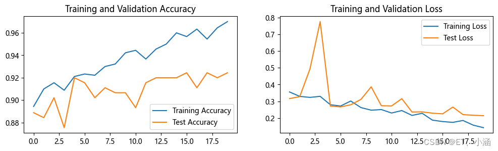： 在这里插入图片描述

从图中我们可以看出训练和测试准确性都随着时间的推移而增加，训练和测试损失都随着时间的推移而减少，说明我们本周构建的模型表现良好，但可能存在轻微的过拟合以及噪声，因为从图中明显能看见几个凸起和凹陷。

七、拔高训练—提高测试集accuracy

1. 我们可以通过增加训练epoch的方法来提高训练集accuracy**

1.1 首先是epoch值为30的情况：

在这里插入图片描述

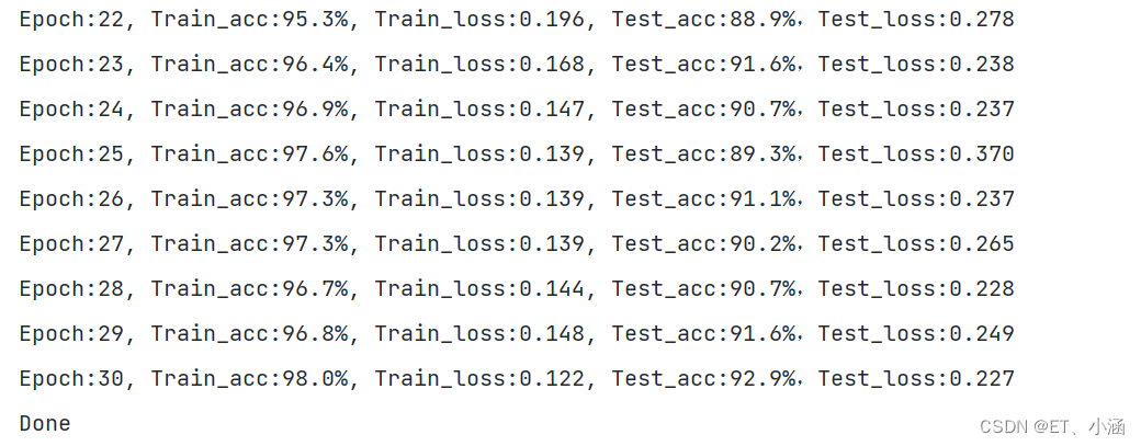
1.2 然后是epoch值为50的情况：

在这里插入图片描述

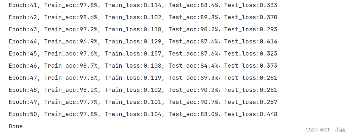
很明显，测试集accuracy得到了提高!

八、碎碎念

1. 我这电脑怎么跑的这么慢啊！！！！！！

2. 突然发现多次训练也可以提高ACcuracy哎。

ET、小涵

关注

19
点赞
踩
22

收藏

觉得还不错? 一键收藏
0
评论
深度学习Week3——天气识别

🍨 本文为🔗365天深度学习训练营中的学习记录博客K同学啊 | 接辅导、项目定制有了前两周的学习，本周内容相对较简单，不过从本周开始，我们的数据集不再使用dataset下载，而是由K同学提供的网盘链接下载到本地，然后从本地当中读取。同时由于我的设备没有GPU，因此直接使用。
复制链接

扫一扫