【深度学习——基于CNN的天气识别】

• 🍨 本文为🔗365天深度学习训练营 中的学习记录博客
• 🍖 原作者：K同学啊 | 接辅导、项目定制
• 🚀 文章来源：K同学的学习圈子

一、前期工作

本文采用CNN实现多云、下雨、晴、日出四种天气状态的识别。

1、设置GPU

import tensorflow as tf


gpus=tf.config.list_physical_devices("GPU")

if gpus:
    gpu0=gpus[0]
    tf.config.experimental.set_memory_growyh(gpu0,True)
    tf.config.set_visible_devices([gpu0],"GPU")
    

2、导入数据

import os,PIL,pathlib
import matplotlib.pyplot as plt
import numpy as np

from tensorflow  import keras
from tensorflow.keras import layers,models

#设置随机数种子
tf.random.set_seed(1)
np.random.seed(1)

data_dir="D:\桌面\深度学习数据\第5天\weather_photos"

data_dir=pathlib.Path(data_dir)

• 随机数种子是一个整数，可以作为随机数生成器的输入，用于确定生成的随机数序列在NumPy库中，可以使用np.random.seed(seed)来设置随机数种子。
  具体来说，np.random.seed(seed)函数用于初始化随机数生成器，并使其生成的随机数序列是确定性的。也就是说，当你使用相同的种子(seed)来调用np.random.seed()时，它会产生相同的随机数序列。这对于复现实验结果和调试代码非常有用。

3、查看数据

image_count=len(list(data_dir.glob('*/*.jpg')))
print("图片总数为：",image_count)

roses=list(data_dir.glob('sunrise/*.jpg'))
PIL.Image.open(str(roses[0]))

实验结果如下图所示：

二、数据预处理

1、加载数据

batch_size = 32
img_height = 180
img_width = 180

"""
关于image_dataset_from_directory()的详细介绍可以参考文章：https://mtyjkh.blog.csdn.net/article/details/117018789
"""
train_ds = tf.keras.preprocessing.image_dataset_from_directory(
    data_dir,
    validation_split=0.2,
    subset="training",
    seed=123,
    image_size=(img_height, img_width),
    batch_size=batch_size)

运行结果如下：

"""
关于image_dataset_from_directory()的详细介绍可以参考文章：https://mtyjkh.blog.csdn.net/article/details/117018789
"""
val_ds = tf.keras.preprocessing.image_dataset_from_directory(
    data_dir,
    validation_split=0.2,
    subset="validation",
    seed=123,
    image_size=(img_height, img_width),
    batch_size=batch_size)

运行结果如下：

2、可视化数据

plt.figure(figsize=(20, 10))
 
for images, labels in train_ds.take(1):
    for i in range(20):
        ax = plt.subplot(5, 10, i + 1)
 
        plt.imshow(images[i].numpy().astype("uint8"))
        plt.title(class_names[labels[i]])
        
        plt.axis("off")

3、再次检查数据

for image_batch, labels_batch in train_ds:
    print(image_batch.shape)
    print(labels_batch.shape)
    break

运行结果如下：

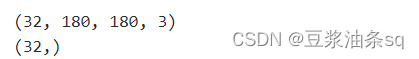
Image_batch是形状的张量(32,180,180,3)。这是一批形状180x180x3的32张图片(最后一维指的是彩色通道RGB)。
Label_batch 是形状(32，）的张量，这些标签对应32张图片

4、配置数据集

• shuffle():打乱数据，关于此函数的详细介绍可以参考：https://zhuanlan.zhihu.com/p/42417456

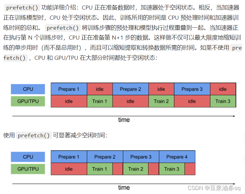
• prefetch():预取数据，加速运行
  

• cache()：将数据集缓存到内存当中，加速运行

AUTOTUNE = tf.data.AUTOTUNE 
train_ds = train_ds.cache().shuffle(1000).prefetch(buffer_size=AUTOTUNE)
val_ds = val_ds.cache().prefetch(buffer_size=AUTOTUNE)

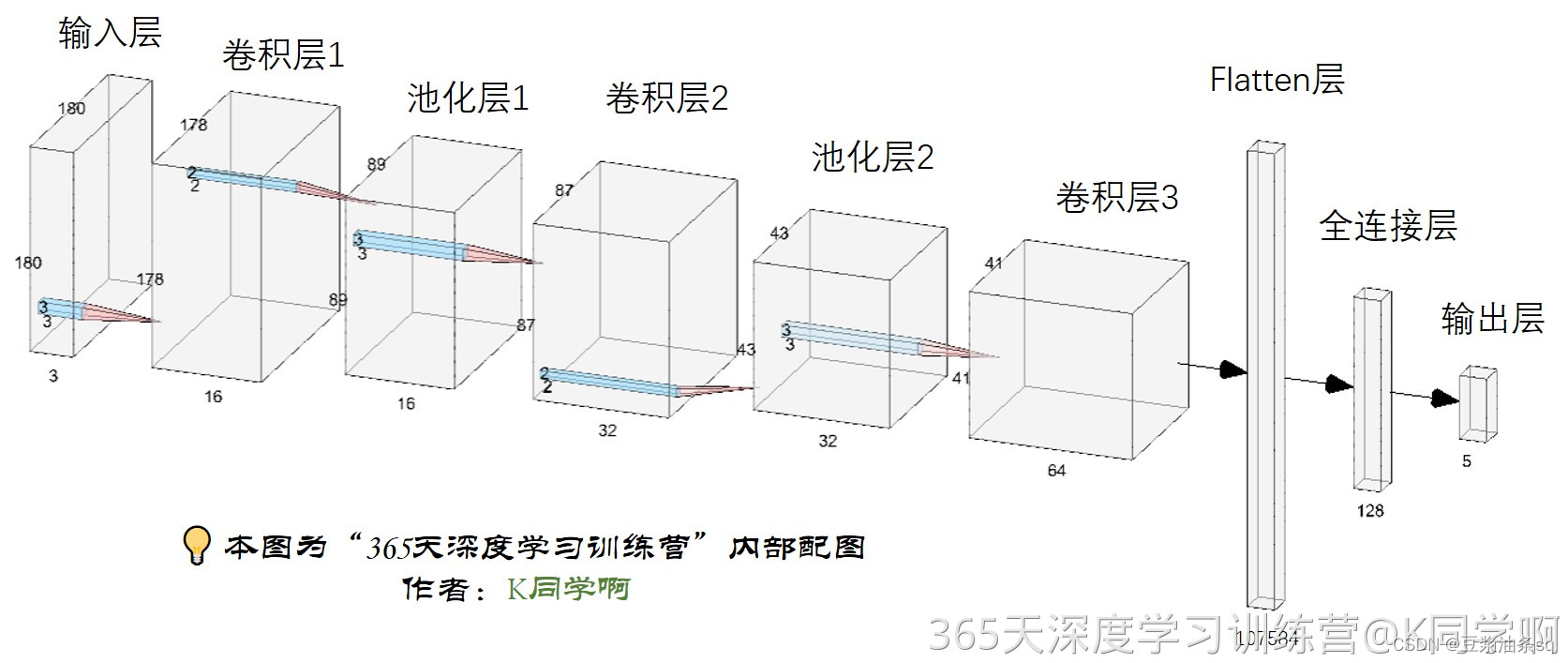
三、构建CNN网络

num_classes = 4
 
"""
关于卷积核的计算不懂的可以参考文章：https://blog.csdn.net/qq_38251616/article/details/114278995
layers.Dropout(0.4) 作用是防止过拟合，提高模型的泛化能力。
在上一篇文章花朵识别中，训练准确率与验证准确率相差巨大就是由于模型过拟合导致的
关于Dropout层的更多介绍可以参考文章：https://mtyjkh.blog.csdn.net/article/details/115826689
"""
 
model = models.Sequential([
    layers.experimental.preprocessing.Rescaling(1./255, input_shape=(img_height, img_width, 3)),
    
    layers.Conv2D(16, (3, 3), activation='relu', input_shape=(img_height, img_width, 3)), # 卷积层1，卷积核3*3  
    layers.AveragePooling2D((2, 2)),               # 池化层1，2*2采样
    layers.Conv2D(32, (3, 3), activation='relu'),  # 卷积层2，卷积核3*3
    layers.AveragePooling2D((2, 2)),               # 池化层2，2*2采样
    layers.Conv2D(64, (3, 3), activation='relu'),  # 卷积层3，卷积核3*3
    layers.Dropout(0.3),  
    
    layers.Flatten(),                       # Flatten层，连接卷积层与全连接层
    layers.Dense(128, activation='relu'),   # 全连接层，特征进一步提取
    layers.Dense(num_classes)               # 输出层，输出预期结果
])
 
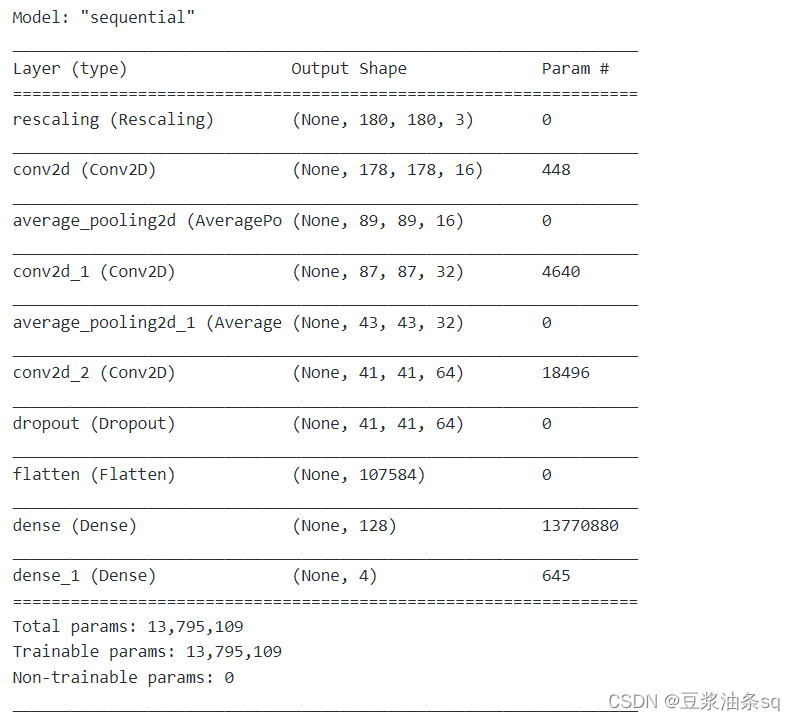
model.summary()  # 打印网络结构

运行结果图如下：

四、编译

使用adma优化器，并设置学习率为0.001

# 设置优化器
opt = tf.keras.optimizers.Adam(learning_rate=0.001)
 
model.compile(optimizer=opt,
              loss=tf.keras.losses.SparseCategoricalCrossentropy(from_logits=True),
              metrics=['accuracy'])

五、训练模型

epochs = 10
 
history = model.fit(
  train_ds,
  validation_data=val_ds,
  epochs=epochs
)

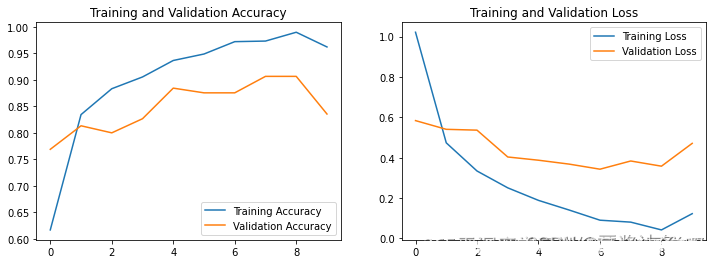
六、模型评估

acc = history.history['accuracy']
val_acc = history.history['val_accuracy']
 
loss = history.history['loss']
val_loss = history.history['val_loss']
 
epochs_range = range(epochs)
 
plt.figure(figsize=(12, 4))
plt.subplot(1, 2, 1)
plt.plot(epochs_range, acc, label='Training Accuracy')
plt.plot(epochs_range, val_acc, label='Validation Accuracy')
plt.legend(loc='lower right')
plt.title('Training and Validation Accuracy')
 
plt.subplot(1, 2, 2)
plt.plot(epochs_range, loss, label='Training Loss')
plt.plot(epochs_range, val_loss, label='Validation Loss')
plt.legend(loc='upper right')
plt.title('Training and Validation Loss')
plt.show()