


目录
1 前言
本文为2021吴恩达学习笔记deeplearning.ai《深度学习专项课程》篇——“第一课——Week3”章节的课后练习,完整内容参见:
深度学习入门指南——2021吴恩达学习笔记deeplearning.ai《深度学习专项课程》篇-CSDN博客
2 基于单隐藏层神经网络的平面数据分类
欢迎来到第三周的编程作业。现在是时候构建你的第一个神经网络了,它将有一个隐藏层。您将看到该模型与使用逻辑回归实现的模型之间的巨大差异。
你将学习如何:
—实现一个具有单个隐藏层的2类分类神经网络;
—使用具有非线性激活功能的单元,如tanh;
—计算交叉熵损失;
—实现正向和反向传播。
2.1 导包
# Package imports
import numpy as np
import matplotlib.pyplot as plt
from testCases_v2 import *
import sklearn
import sklearn.datasets
import sklearn.linear_model
from planar_utils import plot_decision_boundary, sigmoid, load_planar_dataset, load_extra_datasets

%matplotlib inline

np.random.seed(1) # 播下种子,使结果一致
planar_utils.py:
import matplotlib.pyplot as plt
import numpy as np
import sklearn
import sklearn.datasets
import sklearn.linear_model

def plot_decision_boundary(model, X, y):
    # Set min and max values and give it some padding
    x_min, x_max = X[0, :].min() - 1, X[0, :].max() + 1
    y_min, y_max = X[1, :].min() - 1, X[1, :].max() + 1
    h = 0.01
    # Generate a grid of points with distance h between them
    xx, yy = np.meshgrid(np.arange(x_min, x_max, h), np.arange(y_min, y_max, h))
    # Predict the function value for the whole grid
    Z = model(np.c_[xx.ravel(), yy.ravel()])
    Z = Z.reshape(xx.shape)
    # Plot the contour and training examples
    plt.contourf(xx, yy, Z, cmap=plt.cm.Spectral)
    plt.ylabel('x2')
    plt.xlabel('x1')
    plt.scatter(X[0, :], X[1, :], c=y, cmap=plt.cm.Spectral)


def sigmoid(x):
    """
    Compute the sigmoid of x

    Arguments:
    x -- A scalar or numpy array of any size.

    Return:
    s -- sigmoid(x)
    """
    s = 1/(1+np.exp(-x))
    return s

def load_planar_dataset():
    np.random.seed(1)
    m = 400 # number of examples
    N = int(m/2) # number of points per class
    D = 2 # dimensionality
    X = np.zeros((m,D)) # data matrix where each row is a single example
    Y = np.zeros((m,1), dtype='uint8') # labels vector (0 for red, 1 for blue)
    a = 4 # maximum ray of the flower

    for j in range(2):
        ix = range(N*j,N*(j+1))
        t = np.linspace(j*3.12,(j+1)*3.12,N) + np.random.randn(N)*0.2 # theta
        r = a*np.sin(4*t) + np.random.randn(N)*0.2 # radius
        X[ix] = np.c_[r*np.sin(t), r*np.cos(t)]
        Y[ix] = j

    X = X.T
    Y = Y.T

    return X, Y

def load_extra_datasets():
    N = 200
    noisy_circles = sklearn.datasets.make_circles(n_samples=N, factor=.5, noise=.3)
    noisy_moons = sklearn.datasets.make_moons(n_samples=N, noise=.2)
    blobs = sklearn.datasets.make_blobs(n_samples=N, random_state=5, n_features=2, centers=6)
    gaussian_quantiles = sklearn.datasets.make_gaussian_quantiles(mean=None, cov=0.5, n_samples=N, n_features=2, n_classes=2, shuffle=True, random_state=None)
    no_structure = np.random.rand(N, 2), np.random.rand(N, 2)

    return noisy_circles, noisy_moons, blobs, gaussian_quantiles, no_structure
testCases_v2.py:
import numpy as np

def layer_sizes_test_case():
    np.random.seed(1)
    X_assess = np.random.randn(5, 3)
    Y_assess = np.random.randn(2, 3)
    return X_assess, Y_assess

def initialize_parameters_test_case():
    n_x, n_h, n_y = 2, 4, 1
    return n_x, n_h, n_y


def forward_propagation_test_case():
    np.random.seed(1)
    X_assess = np.random.randn(2, 3)
    b1 = np.random.randn(4,1)
    b2 = np.array([[ -1.3]])

    parameters = {'W1': np.array([[-0.00416758, -0.00056267],
        [-0.02136196,  0.01640271],
        [-0.01793436, -0.00841747],
        [ 0.00502881, -0.01245288]]),
     'W2': np.array([[-0.01057952, -0.00909008,  0.00551454,  0.02292208]]),
     'b1': b1,
     'b2': b2}

    return X_assess, parameters

def compute_cost_test_case():
    np.random.seed(1)
    Y_assess = (np.random.randn(1, 3) > 0)
    parameters = {'W1': np.array([[-0.00416758, -0.00056267],
        [-0.02136196,  0.01640271],
        [-0.01793436, -0.00841747],
        [ 0.00502881, -0.01245288]]),
     'W2': np.array([[-0.01057952, -0.00909008,  0.00551454,  0.02292208]]),
     'b1': np.array([[ 0.],
        [ 0.],
        [ 0.],
        [ 0.]]),
     'b2': np.array([[ 0.]])}

    a2 = (np.array([[ 0.5002307 ,  0.49985831,  0.50023963]]))

    return a2, Y_assess, parameters

def backward_propagation_test_case():
    np.random.seed(1)
    X_assess = np.random.randn(2, 3)
    Y_assess = (np.random.randn(1, 3) > 0)
    parameters = {'W1': np.array([[-0.00416758, -0.00056267],
        [-0.02136196,  0.01640271],
        [-0.01793436, -0.00841747],
        [ 0.00502881, -0.01245288]]),
     'W2': np.array([[-0.01057952, -0.00909008,  0.00551454,  0.02292208]]),
     'b1': np.array([[ 0.],
        [ 0.],
        [ 0.],
        [ 0.]]),
     'b2': np.array([[ 0.]])}

    cache = {'A1': np.array([[-0.00616578,  0.0020626 ,  0.00349619],
         [-0.05225116,  0.02725659, -0.02646251],
         [-0.02009721,  0.0036869 ,  0.02883756],
         [ 0.02152675, -0.01385234,  0.02599885]]),
  'A2': np.array([[ 0.5002307 ,  0.49985831,  0.50023963]]),
  'Z1': np.array([[-0.00616586,  0.0020626 ,  0.0034962 ],
         [-0.05229879,  0.02726335, -0.02646869],
         [-0.02009991,  0.00368692,  0.02884556],
         [ 0.02153007, -0.01385322,  0.02600471]]),
  'Z2': np.array([[ 0.00092281, -0.00056678,  0.00095853]])}
    return parameters, cache, X_assess, Y_assess

def update_parameters_test_case():
    parameters = {'W1': np.array([[-0.00615039,  0.0169021 ],
        [-0.02311792,  0.03137121],
        [-0.0169217 , -0.01752545],
        [ 0.00935436, -0.05018221]]),
 'W2': np.array([[-0.0104319 , -0.04019007,  0.01607211,  0.04440255]]),
 'b1': np.array([[ -8.97523455e-07],
        [  8.15562092e-06],
        [  6.04810633e-07],
        [ -2.54560700e-06]]),
 'b2': np.array([[  9.14954378e-05]])}

    grads = {'dW1': np.array([[ 0.00023322, -0.00205423],
        [ 0.00082222, -0.00700776],
        [-0.00031831,  0.0028636 ],
        [-0.00092857,  0.00809933]]),
 'dW2': np.array([[ -1.75740039e-05,   3.70231337e-03,  -1.25683095e-03,
          -2.55715317e-03]]),
 'db1': np.array([[  1.05570087e-07],
        [ -3.81814487e-06],
        [ -1.90155145e-07],
        [  5.46467802e-07]]),
 'db2': np.array([[ -1.08923140e-05]])}
    return parameters, grads

def nn_model_test_case():
    np.random.seed(1)
    X_assess = np.random.randn(2, 3)
    Y_assess = (np.random.randn(1, 3) > 0)
    return X_assess, Y_assess

def predict_test_case():
    np.random.seed(1)
    X_assess = np.random.randn(2, 3)
    parameters = {'W1': np.array([[-0.00615039,  0.0169021 ],
        [-0.02311792,  0.03137121],
        [-0.0169217 , -0.01752545],
        [ 0.00935436, -0.05018221]]),
     'W2': np.array([[-0.0104319 , -0.04019007,  0.01607211,  0.04440255]]),
     'b1': np.array([[ -8.97523455e-07],
        [  8.15562092e-06],
        [  6.04810633e-07],
        [ -2.54560700e-06]]),
     'b2': np.array([[  9.14954378e-05]])}
    return parameters, X_assess
2.2 加载数据集
X, Y = load_planar_dataset()
# 可视化这个数据:
plt.scatter(X[0, :], X[1, :], c=Y, s=40, cmap=plt.cm.Spectral)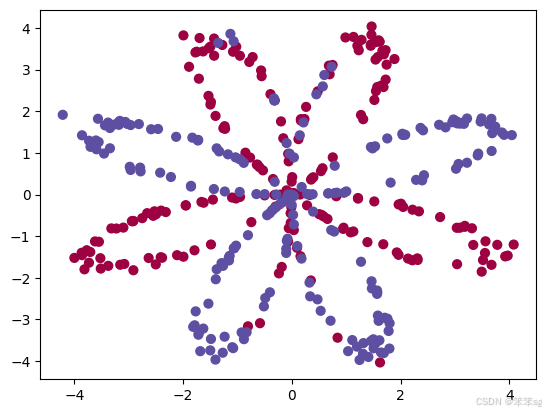
# 获取数据集的数量和形状
shape_X = X.shape
shape_Y = Y.shape
m = (X.size)/shape_X[0]  # training set size

print ('The shape of X is: ' + str(shape_X))
print ('The shape of Y is: ' + str(shape_Y))
print ('I have m = %d training examples!' % (m))
The shape of X is: (2, 400)
The shape of Y is: (1, 400)
I have m = 400 training examples!
2.3 简单的逻辑回归
在建立一个完整的神经网络之前,让我们先看看逻辑回归在这个问题上的表现。可以使用sklearn的内置函数来实现这一点。运行下面的代码来训练数据集上的逻辑回归分类器。
# Train the logistic regression classifier
clf = sklearn.linear_model.LogisticRegressionCV();
clf.fit(X.T, Y.T);
# 绘制这些模型的决策边界
plot_decision_boundary(lambda x: clf.predict(x), X, Y)
plt.title("Logistic Regression")
# 打印准确率
LR_predictions = clf.predict(X.T)
print ('Accuracy of logistic regression: %d ' % float((np.dot(Y,LR_predictions) + np.dot(1-Y,1-LR_predictions))/float(Y.size)*100) +
'% ' + "(percentage of correctly labelled datapoints)")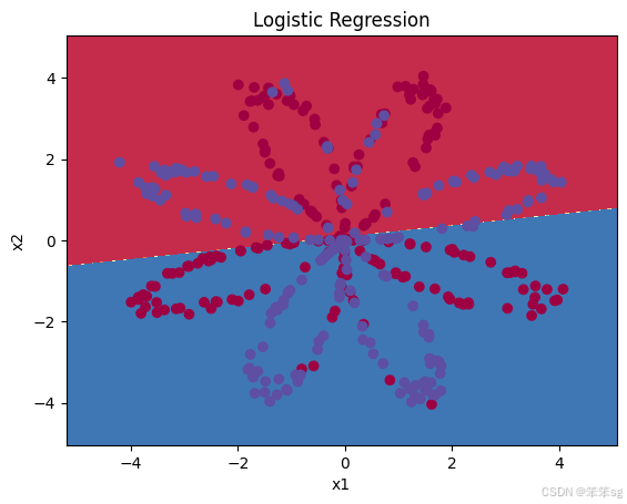
解释:数据集不是线性可分的,所以逻辑回归不表现良好。希望一个神经网络能做得更好。现在让我们试试这个!
2.4 神经网络模型
Logistic回归在“flower dataset”上效果不佳。你要训练一个只有一个隐藏层的神经网络
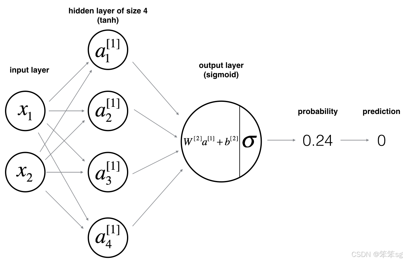
定义神经网络结构
# 定义输入层、隐藏层、输出层的尺寸
def layer_sizes(X, Y):
    n_x = X.shape[0] # size of input layer
    n_h = 4
    n_y = Y.shape[0] # size of output layer
    return (n_x, n_h, n_y)
X_assess, Y_assess = layer_sizes_test_case()
(n_x, n_h, n_y) = layer_sizes(X_assess, Y_assess)
print("The size of the input layer is: n_x = " + str(n_x))
print("The size of the hidden layer is: n_h = " + str(n_h))
print("The size of the output layer is: n_y = " + str(n_y))
The size of the input layer is: n_x = 5
The size of the hidden layer is: n_h = 4
The size of the output layer is: n_y = 2
初始化模型参数
def initialize_parameters(n_x, n_h, n_y):
    """
    W1 -- weight matrix of shape (n_h, n_x)
    b1 -- bias vector of shape (n_h, 1)
    W2 -- weight matrix of shape (n_y, n_h)
    b2 -- bias vector of shape (n_y, 1)
    """

    np.random.seed(2) # 虽然初始化是随机的,但我们设置了一个种子,以便您的输出与我们的输出匹配。

    W1 = np.random.randn(n_h,n_x) * 0.01
    b1 = np.zeros((n_h,1))
    W2 = np.random.randn(n_y,n_h) * 0.01
    b2 = np.zeros((n_y,1))

    assert (W1.shape == (n_h, n_x))
    assert (b1.shape == (n_h, 1))
    assert (W2.shape == (n_y, n_h))
    assert (b2.shape == (n_y, 1))

    parameters = {"W1": W1,
                  "b1": b1,
                  "W2": W2,
                  "b2": b2}

    return parameters

n_x, n_h, n_y = initialize_parameters_test_case()

parameters = initialize_parameters(n_x, n_h, n_y)
print("W1 = " + str(parameters["W1"]))
print("b1 = " + str(parameters["b1"]))
print("W2 = " + str(parameters["W2"]))
print("b2 = " + str(parameters["b2"]))
W1 = [[-0.00416758 -0.00056267]
[-0.02136196 0.01640271]
[-0.01793436 -0.00841747]
[ 0.00502881 -0.01245288]]
b1 = [[0.]
[0.]
[0.]
[0.]]
W2 = [[-0.01057952 -0.00909008 0.00551454 0.02292208]]
b2 = [[0.]]
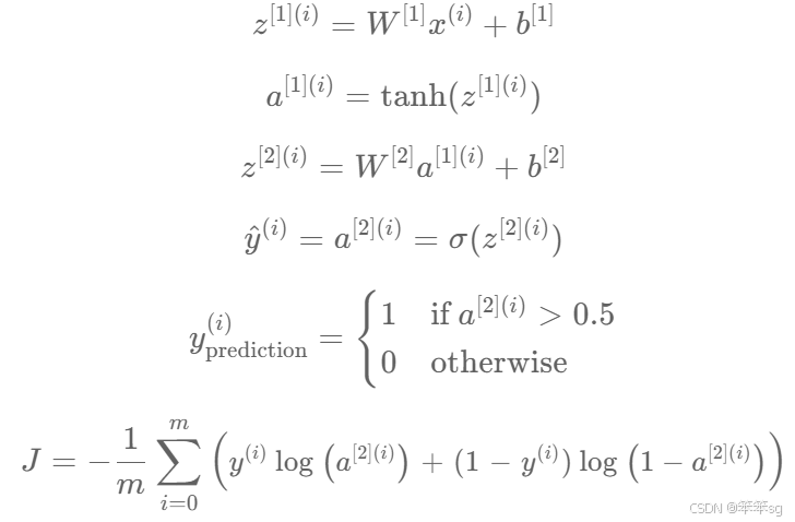
前向传播和反向传播
# GRADED FUNCTION: forward_propagation

def forward_propagation(X, parameters):
    # 从字典“parameters”中检索每个参数
    W1 = parameters["W1"]
    b1 = parameters["b1"]
    W2 = parameters["W2"]
    b2 = parameters["b2"]

    # 实现前向传播来计算A2(概率)
    Z1 = np.dot(W1,X) + b1
    A1 = np.tanh(Z1)
    Z2 = np.dot(W2,A1) + b2
    A2 = sigmoid(Z2)

    assert(A2.shape == (1, X.shape[1]))

    # 反向传播所需的值存储在“缓存”中。这将作为反向传播的输入
    cache = {"Z1": Z1,
             "A1": A1,
             "Z2": Z2,
             "A2": A2}

    return A2, cache
X_assess, parameters = forward_propagation_test_case()
A2, cache = forward_propagation(X_assess, parameters)

# 注意:我们在这里使用平均值只是为了确保你的输出与我们的匹配。
print(
    np.mean(cache["Z1"]),
    np.mean(cache["A1"]),
    np.mean(cache["Z2"]),
    np.mean(cache["A2"]),
)
0.26281864019752443 0.09199904522700109 -1.3076660128732143 0.21287768171914198
# GRADED FUNCTION: compute_cost

def compute_cost(A2, Y, parameters):
    m = Y.shape[1] # 样本数量

    # 计算二元交叉熵损失
    logprobs = logprobs = np.multiply(Y ,np.log(A2)) + np.multiply((1-Y), np.log(1-A2))
    cost = (-1/m) * np.sum(logprobs)
    cost = float(np.squeeze(cost))
    assert(isinstance(cost, float))

    return cost
A2, Y_assess, parameters = compute_cost_test_case()

print("cost = " + str(compute_cost(A2, Y_assess, parameters)))
cost = 0.6930587610394646
使用前向传播期间计算的缓存,现在可以实现后向传播。
反向传播通常是深度学习中最难(最数学化)的部分。
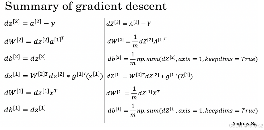
# GRADED FUNCTION: backward_propagation

def backward_propagation(parameters, cache, X, Y):
    m = X.shape[1]

    # 首先,从字典“parameters”中检索W1和W2。
    W1 = parameters["W1"]
    b1 = parameters["b1"]
    W2 = parameters["W2"]
    b2 = parameters["b2"]

    # 接着从字典“cache”中检索A1和A2。
    A1 = cache["A1"]
    A2 = cache["A2"]
    Z1 = cache["Z1"]
    Z2 = cache["Z2"]

    # 反向传播:计算dW1、db1、dW2、db2。
    dZ2 = A2 - Y
    dW2 = (1/m) * np.dot(dZ2,A1.T)
    db2 = (1/m) *(np.sum(dZ2,axis=1,keepdims=True))
    dZ1 = np.dot(W2.T,dZ2) * (1 - np.power(A1,2))
    dW1 = (1/m) *(np.dot(dZ1,X.T))
    db1 = (1/m) *(np.sum(dZ1, axis=1, keepdims=True))

    grads = {"dW1": dW1,
             "db1": db1,
             "dW2": dW2,
             "db2": db2}

    return grads
parameters, cache, X_assess, Y_assess = backward_propagation_test_case()

grads = backward_propagation(parameters, cache, X_assess, Y_assess)
print("dW1 = " + str(grads["dW1"]))
print("db1 = " + str(grads["db1"]))
print("dW2 = " + str(grads["dW2"]))
print("db2 = " + str(grads["db2"]))
dW1 = [[ 0.00301023 -0.00747267]
[ 0.00257968 -0.00641288]
[-0.00156892 0.003893 ]
[-0.00652037 0.01618243]]
db1 = [[ 0.00176201]
[ 0.00150995]
[-0.00091736]
[-0.00381422]]
dW2 = [[ 0.00078841 0.01765429 -0.00084166 -0.01022527]]
db2 = [[-0.16655712]]
参数更新
# GRADED FUNCTION: update_parameters

def update_parameters(parameters, grads, learning_rate):
    # 从字典“parameters”中检索每个参数
    W1 = parameters["W1"]
    b1 = parameters["b1"]
    W2 = parameters["W2"]
    b2 = parameters["b2"]

    # 从字典“gradients”中检索每个梯度
    dW1 = grads["dW1"]
    db1 = grads["db1"]
    dW2 = grads["dW2"]
    db2 = grads["db2"]

    # 更新每个参数
    W1 = W1 - learning_rate * dW1
    b1 = b1 - learning_rate * db1
    W2 = W2 - learning_rate * dW2
    b2 = b2 - learning_rate * db2

    parameters = {"W1": W1,
                  "b1": b1,
                  "W2": W2,
                  "b2": b2}

    return parameters
parameters, grads = update_parameters_test_case()
parameters = update_parameters(parameters, grads, 1.2)

print("W1 = " + str(parameters["W1"]))
print("b1 = " + str(parameters["b1"]))
print("W2 = " + str(parameters["W2"]))
print("b2 = " + str(parameters["b2"]))
W1 = [[-0.00643025 0.01936718]
[-0.02410458 0.03978052]
[-0.01653973 -0.02096177]
[ 0.01046864 -0.05990141]]
b1 = [[-1.02420756e-06]
[ 1.27373948e-05]
[ 8.32996807e-07]
[-3.20136836e-06]]
W2 = [[-0.01041081 -0.04463285 0.01758031 0.04747113]]
b2 = [[0.00010457]]
将各个模块合并至模型中
# NN_model
def nn_model(X, Y, n_h, learning_rate, num_iterations = 10000, print_cost=False):
    n_x = layer_sizes(X, Y)[0]
    n_y = layer_sizes(X, Y)[2]

    # 初始化参数
    parameters = initialize_parameters(n_x, n_h, n_y)
    W1 = parameters["W1"]
    b1 = parameters["b1"]
    W2 = parameters["W2"]
    b2 = parameters["b2"]

    # 循环(梯度下降)
    for i in range(0, num_iterations):
        # 前向传播
        A2, cache = forward_propagation(X, parameters)
        # 计算代价
        cost = compute_cost(A2, Y, parameters)
        # 反向传播,计算梯度
        grads = backward_propagation(parameters, cache, X, Y)
        # 更新参数
        parameters = update_parameters(parameters, grads, learning_rate)
        # 打印每1000次迭代的成本
        if print_cost and i % 1000 == 0:
            print ("Cost after iteration %i: %f" %(i, cost))
    # 返回模型学习到的参数。然后,它们可以用来预测输出
    return parameters

X_assess, Y_assess = nn_model_test_case()
parameters = nn_model(X_assess, Y_assess, 4, 1.02,num_iterations=10000, print_cost=True)
print("W1 = " + str(parameters["W1"]))
print("b1 = " + str(parameters["b1"]))
print("W2 = " + str(parameters["W2"]))
print("b2 = " + str(parameters["b2"]))
Cost after iteration 0: 0.692739
Cost after iteration 1000: 0.000257
Cost after iteration 2000: 0.000127
Cost after iteration 3000: 0.000084
Cost after iteration 4000: 0.000063
Cost after iteration 5000: 0.000050
Cost after iteration 6000: 0.000042
Cost after iteration 7000: 0.000036
Cost after iteration 8000: 0.000031
Cost after iteration 9000: 0.000028
W1 = [[-0.65400312 1.21068652]
[-0.75688005 1.38443617]
[ 0.57449374 -1.0957478 ]
[ 0.76242342 -1.40517716]]
b1 = [[ 0.2841426 ]
[ 0.34699428]
[-0.23981061]
[-0.35351855]]
W2 = [[-2.42329584 -3.22274999 1.97978376 3.31771228]]
b2 = [[0.20282644]]
预测
# GRADED FUNCTION: predict

def predict(parameters, X):
    A2, cache = forward_propagation(X, parameters)
    predictions = (A2 > 0.5)

    return predictions
parameters, X_assess = predict_test_case()

predictions = predict(parameters, X_assess)
print("predictions mean = " + str(np.mean(predictions)))
predictions mean = 0.6666666666666666
是时候运行这个模型了,看看它在平面数据集上的表现如何。
# 建立一个具有n_h维隐藏层的模型
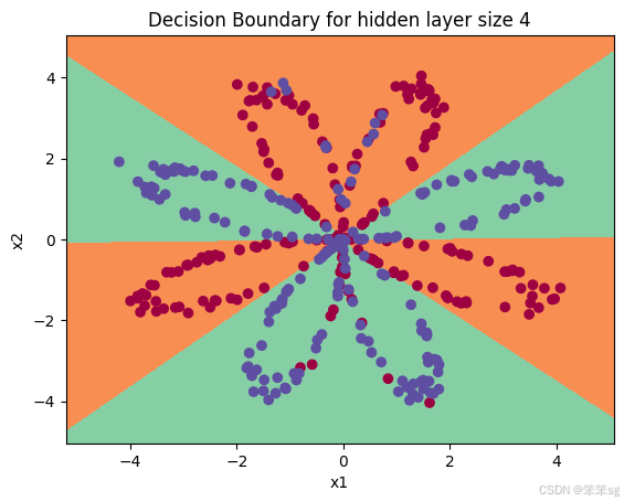
parameters = nn_model(X, Y, 4, 1.2 , num_iterations = 10000, print_cost=True)
# 绘制决策边界
plot_decision_boundary(lambda x: predict(parameters, x.T), X, Y)
plt.title("Decision Boundary for hidden layer size " + str(4))Cost after iteration 0: 0.693048
Cost after iteration 1000: 0.288083
Cost after iteration 2000: 0.254385
Cost after iteration 3000: 0.233864
Cost after iteration 4000: 0.226792
Cost after iteration 5000: 0.222644
Cost after iteration 6000: 0.219731
Cost after iteration 7000: 0.217504
Cost after iteration 8000: 0.219440
Cost after iteration 9000: 0.218553
# 打印准确率
predictions = predict(parameters, X)
print ('Accuracy: %d' % float((np.dot(Y,predictions.T) + np.dot(1-Y,1-predictions.T))/float(Y.size)*100) + '%')
Accuracy: 90%
与逻辑回归相比,准确率真的很高。模特已经学会了花的叶子图案!与逻辑回归不同,神经网络甚至能够学习高度非线性的决策边界。
现在,让我们尝试几种隐藏层的大小。
调整隐藏层大小
运行以下代码。可能需要1-2分钟。您将观察到不同隐藏层大小的模型的不同行为。
# This may take about 2 minutes to run

plt.figure(figsize=(16, 32))
hidden_layer_sizes = [1, 2, 3, 4, 5, 20, 50]
for i, n_h in enumerate(hidden_layer_sizes):
    plt.subplot(5, 2, i+1)
    plt.title('Hidden Layer of size %d' % n_h)
    parameters = nn_model(X, Y, n_h,1.2, num_iterations = 5000)
    plot_decision_boundary(lambda x: predict(parameters, x.T), X, Y)
    predictions = predict(parameters, X)
    accuracy = float((np.dot(Y,predictions.T) + np.dot(1-Y,1-predictions.T))/float(Y.size)*100)
    print ("Accuracy for {} hidden units: {} %".format(n_h, accuracy))
Accuracy for 1 hidden units: 67.5 %
Accuracy for 2 hidden units: 67.25 %
Accuracy for 3 hidden units: 90.75 %
Accuracy for 4 hidden units: 90.5 %
Accuracy for 5 hidden units: 91.25 %
Accuracy for 20 hidden units: 90.5 %
Accuracy for 50 hidden units: 90.25 %
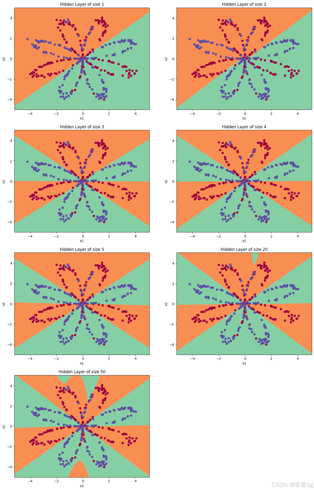
释意:
- 较大的模型(有更多隐藏单元)能够更好地拟合训练集,直到最终最大的模型过拟合数据。
- 最好的隐藏层大小似乎是在n_h = 5左右。实际上,这里的值似乎很适合数据,而不会引起明显的过拟合。
- 稍后您还将学习正则化,它允许您使用非常大的模型(例如n_h = 50)而不会过度拟合。
2.5 其他数据集上的性能
# Datasets
noisy_circles, noisy_moons, blobs, gaussian_quantiles, no_structure = load_extra_datasets()

datasets = {"noisy_circles": noisy_circles,
            "noisy_moons": noisy_moons,
            "blobs": blobs,
            "gaussian_quantiles": gaussian_quantiles}

dataset = "noisy_moons"

X, Y = datasets[dataset]
X, Y = X.T, Y.reshape(1, Y.shape[0])

# make blobs binary
if dataset == "blobs":
    Y = Y%2

# 可视化数据
plt.scatter(X[0, :], X[1, :], c=Y.reshape(200), s=40, cmap=plt.cm.Spectral)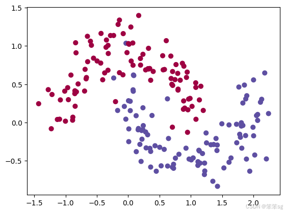
parameters = nn_model(X, Y, n_h, 1.2, num_iterations=5000)
plot_decision_boundary(lambda x: predict(parameters, x.T), X, Y)

predictions = predict(parameters, X)
accuracy = float(
    (np.dot(Y, predictions.T) + np.dot(1 - Y, 1 - predictions.T)) / float(Y.size) * 100
)
print("Accuracy: ", accuracy)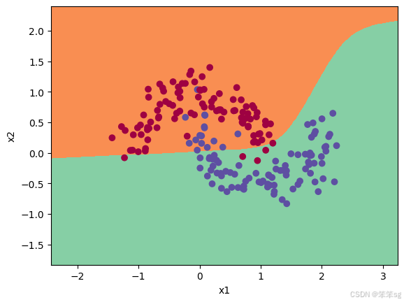


 1096
1096

 被折叠的 条评论
为什么被折叠?
被折叠的 条评论
为什么被折叠?
 到【灌水乐园】发言


