特征选择

1. 简介

特征选择是一个很重要的数据预处理过程：

• 选择出重要的特征可以缓解维数灾难问题
• 去除不相关特征可以降低学习任务的难度

特征选择可分为子集搜索和子集评价：

• 子集搜索：前向搜索（逐渐增加特征），后向搜索（逐渐减少特征）
• 子集评价：可采用信息增益对子集进行评价

特征选择的方式有：

• 包裹式选择
• 过滤式选择
• 嵌入式选择

---

2. 包裹式（封装器法）

包裹式（封装器法）从初始特征集合中不断的选择特征子集，训练学习器，根据学习器的性能来对子集进行评价，直到选择出最佳的子集。包裹式特征选择直接针对给定学习器进行优化

2.1 循环特征选择

常用实现方法：循序特征选择。

• 循序向前特征选择：Sequential Forward Selection，SFS
• 循序向后特征选择：Sequential Backword Selection，SBS

SFS过程如下：

#加载数据集
from mlxtend.feature_selection import SequentialFeatureSelector as SFS #SFS
from mlxtend.data import wine_data #dataset
from sklearn.neighbors import KNeighborsClassifier
from sklearn.model_selection import train_test_split
from sklearn.preprocessing import StandardScaler

X, y = wine_data()
X.shape  #(178, 13)

#数据预处理
X_train, X_test, y_train, y_test= train_test_split(X, y, stratify=y, test_size=0.3, random_state=1)
std = StandardScaler()
X_train_std = std.fit_transform(X_train)

#循序向前特征选择
knn = KNeighborsClassifier(n_neighbors=3)

sfs = SFS(estimator=knn, k_features=4, forward=True, floating=False, verbose=2, scoring='accuracy', cv=0)
sfs.fit(X_train_std, y_train)  #xy不能是df

#查看特征索引
sfs.subsets_

可视化1

%matplotlib inline
from mlxtend.plotting import plot_sequential_feature_selection as plot_sfs
fig = plot_sfs(sfs.get_metric_dict(), kind='std_err') 

查看 sfs.get_metric_dict()结果

可视化2

knn = KNeighborsClassifier(n_neighbors=3)
sfs2 = SFS(estimator=knn, k_features=(3, 10),
                   forward=True, 
                   floating=True,   
                   verbose=0,
                   scoring='accuracy',
                   cv=5)
sfs2.fit(X_train_std, y_train)
fig = plot_sfs(sfs2.get_metric_dict(), kind='std_err')

2.2 穷举特征选择

穷举特征选择（Exhaustive feature selection），即封装器中搜索算法是将所有特征组合都实现一遍，然后通过比较各种特征组合后的模型表现，从中选择出最佳的特征子集

这里用到是鸢尾花数据集，该数据集有四个特征，那么穷举产生的特征组合个数为15

#导入相关库
from mlxtend.feature_selection import ExhaustiveFeatureSelector as EFS
from sklearn.neighbors import KNeighborsClassifier
from sklearn.datasets import load_iris

#加载数据集
iris = load_iris()
X = iris.data
y = iris.target

#穷举特征选择
knn = KNeighborsClassifier(n_neighbors=3) # n_neighbors=3

efs = EFS(knn,
         min_features=1,
         max_features=4,
         scoring='accuracy',
         print_progress=True,
         cv=5)
efs = efs.fit(X, y)

#查看最佳特征子集
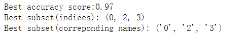
print('Best accuracy score: %.2f' % efs.best_score_)  #Best accuracy score: 0.97
print('Best subset(indices):', efs.best_idx_)         #Best subset(indices): (0, 2, 3)
print('Best subset (correponding names):', efs.best_feature_names_)  #没有这个函数 

#度量标准
efs.get_metric_dict()


import pandas as pd

df = pd.DataFrame.from_dict(efs.get_metric_dict()).T
df.sort_values('avg_score', inplace=True, ascending=False)
df

#可视化
import matplotlib.pyplot as plt 

#平均值
metric_dict=efs.get_metric_dict()
k_feat=sorted(metric_dict.keys())
print('k_feat:',k_feat)
avg=[metric_dict[k]['avg_score']for k in k_feat]


#绘制区域图区域，平均值+-标准差
fig=plt.figure()
upper,lower=[],[]
for k in k_feat: #bound
    upper.append(metric_dict[k]['avg_score'] + metric_dict[k]['std_dev']) 
    lower.append(metric_dict[k]['avg_score'] - metric_dict[k]['std_dev'])
    
plt.fill_between(k_feat,upper,lower,alpha=0.2,color='blue',lw=1)
plt.show()
plt.close()

#绘制折线图
plt.plot(k_feat,avg,color='blue',marker='o')

---

3. 过滤器法

• 方差阈值（VarianceThreshold）
• （SelectBest）

3.1 方差阈值

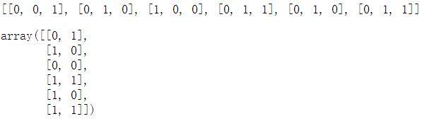
方差阈值（VarianceThreshold）是特征选择的一个简单方法，去掉那些方差没有达到阈值的特征。默认情况下，删除零方差的特征，例如那些只有一个值的样本。
假设我们有一个有布尔特征的数据集，然后我们想去掉那些超过80%的样本都是0（或者1）的特征。布尔特征是伯努利随机变量，方差为 p(1-p)。

使用方差选择法，先要计算各个特征的方差，然后根据阈值，选择方差大于阈值的特征。使用feature_selection库的VarianceThreshold类
方差选择法，返回值为特征选择后的数据 #参数threshold为方差的阈值

from sklearn.feature_selection import VarianceThreshold
X = [[0, 0, 1], [0, 1, 0], [1, 0, 0], [0, 1, 1], [0, 1, 0], [0, 1, 1]]
print(X)  

sel=VarianceThreshold(threshold=(.8*(1-.8)))
sel.fit_transform(X,y)

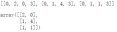
X = [[0, 2, 0, 3], [0, 1, 4, 3], [0, 1, 1, 3]]
print(X)  #[[0, 2, 0, 3], [0, 1, 4, 3], [0, 1, 1, 3]]

seletor = VarianceThreshold()  #默认方法大于0
seletor.fit_transform(X)

'''
0203
0143
0113
'''

嵌入法

对系数排序——即特征权重，然后依据某个阈值选择部分特征。
在训练模型的同时，得到了特征权重，并完成特征选择。像这样，将特征选择过程与模型训练融为一体，在模型训练过程中自动进行了特征选择，被称为“嵌入法” （Embedded）特征选择。

在过滤式和包裹式特征选择方法中，特征选择过程与学习器训练过程有明显的分别。而嵌入式特征选择在学习器训练过程中自动地进行特征选择。

嵌入式选择最常用的是L1正则化与L2正则化。在对线性回归模型加入两种正则化方法后，他们分别变成了岭回归与Lasso回归

xgboost自带feature_importances_

例子1

使用xgb对鸢尾花数据集进行预测，并绘制重要性表格

##例子1
#加载鸢尾花数据集
iris = load_iris()
X = iris.data
y = iris.target

#Xgboost特征重要性
from xgboost import XGBClassifier
model = XGBClassifier() # 分类
model.fit(X,y)
model.feature_importances_  # 特征重要性  array([0.01251974, 0.03348068, 0.59583396, 0.35816565], dtype=float32)

#可视化
%matplotlib inline
from xgboost import plot_importance
plot_importance(model)

例子2
使用Lasso回归对波士顿房价进行预测

import matplotlib.pyplot as plt
import numpy as np

from sklearn.datasets import load_boston
from sklearn.feature_selection import SelectFromModel
from sklearn.linear_model import LassoCV

# Load the boston dataset.
X, y = load_boston(return_X_y=True)

# We use the base estimator LassoCV since the L1 norm promotes sparsity of features.
clf = LassoCV()

# Set a minimum threshold of 0.25
sfm = SelectFromModel(clf, threshold=0.25)
sfm.fit(X, y)
n_features = sfm.transform(X).shape[1]

# Reset the threshold till the number of features equals two.
# Note that the attribute can be set directly instead of repeatedly
# fitting the metatransformer.
while n_features > 2:
    sfm.threshold += 0.1
    X_transform = sfm.transform(X)
    n_features = X_transform.shape[1]
# Plot the selected two features from X.
plt.title(
"Features selected from Boston using SelectFromModel with " "threshold %0.3f." % sfm.threshold)
feature1 = X_transform[:, 0]
feature2 = X_transform[:, 1]
plt.plot(feature1, feature2, 'r.')
plt.xlabel("Feature number 1")
plt.ylabel("Feature number 2")
plt.ylim([np.min(feature2), np.max(feature2)])
plt.show()

参考文献

• https://www.cnblogs.com/cgmcoding/p/13523501.html