


目录
学习率敏感度
上一次构建带bn层的神经网络中,会发现一个现象,加入bn层不会提升模型迭代的平稳性,甚至加入bn层后模型不平稳的特点会更严重。不平稳性一般与学习率有关,为了解决这一现象,我们可以对学习率进行优化调整。我们先观察学习率与模型不平稳之间的关系(在学习率分别为0.1,0.01,0.03,0.005时,模型的误差变化情况):
def test_lr():
    utils = MyTorchUtils()
    torch.manual_seed(929)

    # create data
    feature,labels = utils.tensorDataGenRe(bag=2,w=[2,-1,3,1,2],bias=False)

    # split data
    train_loader,test_loader = utils.split_loader(feature,labels,batch_size=50)

    tanh_model3 = net_class3(act_fun=torch.tanh,in_features=5)
    tanh_model3_norml = net_class3(act_fun=torch.tanh,in_features=5,BN_model='pre')
    tanh_model4 = net_class4(act_fun=torch.tanh,in_features=5)
    tanh_model4_norml = net_class4(act_fun=torch.tanh,in_features=5,BN_model='pre')

    model_1 = [tanh_model3,tanh_model3_norml,tanh_model4,tanh_model4_norml]
    name_1 = ['tanh_model3','tanh_model3_norml','tanh_model4','tanh_model4_norml']

    num_epochs = 40

    train_01,test_01 = utils.model_comparison(model_1=model_1,name_1=name_1,
                                              train_data=train_loader,
                                              test_data=test_loader,
                                              num_epochs=num_epochs,
                                              optimizer=optim.SGD,
                                              criterion=nn.MSELoss(),
                                              lr=0.1,cla=False,
                                              eva=utils.mse_cla)

    tanh_model3 = net_class3(act_fun=torch.tanh, in_features=5)
    tanh_model3_norml = net_class3(act_fun=torch.tanh, in_features=5, BN_model='pre')
    tanh_model4 = net_class4(act_fun=torch.tanh, in_features=5)
    tanh_model4_norml = net_class4(act_fun=torch.tanh, in_features=5, BN_model='pre')

    model_1 = [tanh_model3, tanh_model3_norml, tanh_model4, tanh_model4_norml]
    name_1 = ['tanh_model3', 'tanh_model3_norml', 'tanh_model4', 'tanh_model4_norml']

    train_003, test_003 = utils.model_comparison(model_1=model_1, name_1=name_1,
                                                 train_data=train_loader,
                                                 test_data=test_loader,
                                                 num_epochs=num_epochs,
                                                 optimizer=optim.SGD,
                                                 criterion=nn.MSELoss(),
                                                 lr=0.03, cla=False,
                                                 eva=utils.mse_cla)

    tanh_model3 = net_class3(act_fun=torch.tanh, in_features=5)
    tanh_model3_norml = net_class3(act_fun=torch.tanh, in_features=5, BN_model='pre')
    tanh_model4 = net_class4(act_fun=torch.tanh, in_features=5)
    tanh_model4_norml = net_class4(act_fun=torch.tanh, in_features=5, BN_model='pre')

    model_1 = [tanh_model3, tanh_model3_norml, tanh_model4, tanh_model4_norml]
    name_1 = ['tanh_model3', 'tanh_model3_norml', 'tanh_model4', 'tanh_model4_norml']

    train_001, test_001 = utils.model_comparison(model_1=model_1, name_1=name_1,
                                                 train_data=train_loader,
                                                 test_data=test_loader,
                                                 num_epochs=num_epochs,
                                                 optimizer=optim.SGD,
                                                 criterion=nn.MSELoss(),
                                                 lr=0.01, cla=False,
                                                 eva=utils.mse_cla)

    tanh_model3 = net_class3(act_fun=torch.tanh, in_features=5)
    tanh_model3_norml = net_class3(act_fun=torch.tanh, in_features=5, BN_model='pre')
    tanh_model4 = net_class4(act_fun=torch.tanh, in_features=5)
    tanh_model4_norml = net_class4(act_fun=torch.tanh, in_features=5, BN_model='pre')

    model_1 = [tanh_model3, tanh_model3_norml, tanh_model4, tanh_model4_norml]
    name_1 = ['tanh_model3', 'tanh_model3_norml', 'tanh_model4', 'tanh_model4_norml']

    train_0005, test_0005 = utils.model_comparison(model_1=model_1, name_1=name_1,
                                                   train_data=train_loader,
                                                   test_data=test_loader,
                                                   num_epochs=num_epochs,
                                                   optimizer=optim.SGD,
                                                   criterion=nn.MSELoss(),
                                                   lr=0.005, cla=False,
                                                   eva=utils.mse_cla)

    plt.subplot(221)
    for i,name in enumerate(name_1):
        plt.plot(list(range(num_epochs)),train_01[i])


    plt.subplot(222)
    for i,name in enumerate(name_1):
        plt.plot(list(range(num_epochs)),train_003[i])


    plt.subplot(223)
    for i,name in enumerate(name_1):
        plt.plot(list(range(num_epochs)),train_001[i])


    plt.subplot(224)
    for i, name in enumerate(name_1):
        plt.plot(list(range(num_epochs)), train_0005[i],label=name)
    plt.legend(loc=1)
    plt.show()
代码要注意的一个,我们每次训练时都要重新定义一个全新的网络
结果
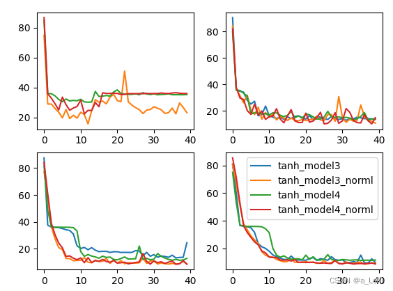
由上图我们基本可以得出结论,学习率的变化会嚷有bn层的模型有较大的波动,即有bn层的模型对学习率变化更加敏感,而对于此类模型而言,调整学习率往往会获得更好的效果。
学习率的学习曲线
从上面的结果看出,当学习率越小的时候,模型表现越稳定。实际情况可能是,当学习率较大时,模型会在最优点附近来回振荡,但由于步长过大,一直跨过最优点。而学习率较小时会解决这个情况,但也会存在过小导致步长太短无法走到最优点的情况。所以学习率的学习曲线就像是"随着学习率降低,模型的损失越来越小,到最小点后,学习率越小,损失反而会越来越大的U形图像"。可以用我上面的代码去证明。
常用的学习率调度策略
幂调度:lr -- lr/2 -- lr/3
指数调度:lr -- lr/10^1 -- lr/10^2
分段恒定调度:每间隔一段时间调整一小学习率,比如1~100为lr,100~200为lr/100.
性能调度:每隔一段时间观察误差变化情况,误差不变,则降低学习率继续迭代
周期调度:学习率在一个周期内进行先递增后递减的变化
学习率调度在pytorch中的实现方法
让优化器动态调整学习率的类称为学习率调度器类,所有学习率调度器中,lambdaLR是最通用的一种方法。
from torch.optim import lr_scheduler
import torch.nn as nn
import torch

# Create lambda function
lr_lambda = lambda  epoch: 0.5 ** epoch

class net_class2(nn.Module):
    def __init__(self,act_fun=torch.relu,in_features=2,n_hidden1=4,n_hidden2=4,out_features=1,bias=True,BN_model=None,momentum=0.1):
        super(net_class2, self).__init__()
        self.linear1 = nn.Linear(in_features,n_hidden1,bias=bias)
        self.bn1 = nn.BatchNorm1d(n_hidden1,momentum=momentum)
        self.linear2 = nn.Linear(n_hidden1,n_hidden2,bias=bias)
        self.bn2 = nn.BatchNorm1d(n_hidden2,momentum=momentum)
        self.linear3 = nn.Linear(n_hidden2,out_features,bias=bias)
        self.act_fun = act_fun
        self.BN_model = BN_model

    def forward(self,x):
        if self.BN_model == 'pre':
            z1 = self.bn1(self.linear1(x))
            f1 = self.act_fun(z1)
            z2 = self.bn2(self.linear2(f1))
            out = self.linear3(self.act_fun(z2))

        elif self.BN_model == 'post':
            z1 = self.linear1(x)
            f1 = self.act_fun(z1)
            z2 = self.linear2(self.bn1(f1))
            f2 = self.act_fun(z2)
            out = self.linear3(self.bn2(f2))
        else:
            z1 = self.linear1(x)
            f1 = self.act_fun(z1)
            z2 = self.linear2(f1)
            out = self.linear3(self.act_fun(z2))
        return out

torch.manual_seed(422)

tahn_model1 = net_class2(act_fun=torch.tanh,in_features=5,BN_model='pre')

optimizer = torch.optim.SGD(tahn_model1.parameters(),lr=0.05)

# print(optimizer.state_dict())

# Create Learning Rate Scheduler
scheduler = lr_scheduler.LambdaLR(optimizer,lr_lambda)

print(optimizer.state_dict())
结果如下:
{'state': {}, 'param_groups': [{'lr': 0.05, 'momentum': 0, 'dampening': 0, 'weight_decay': 0, 'nesterov': False, 'initial_lr': 0.05, 'params': [0, 1, 2, 3, 4, 5, 6, 7, 8, 9]}]}其中intiial_lr代表最初的lr值,lr代表下一轮要进行训练时lr的值,根据设置的调度器的计算方法,lr的更新规为new_lr = lr_lambda(epoch) * initial_lr。
更新lr:
for X,y in train_loader:
    yhat = tahn_model1.forward(X)
    loss = criterion(yhat,y)
    optimizer.zero_grad()
    loss.backward()
    optimizer.step()
scheduler.step()
此时,数据训练了一次,epoch=1,lr更新为0.025.


 812
812


 被折叠的 条评论
为什么被折叠?
被折叠的 条评论
为什么被折叠?
 到【灌水乐园】发言


