机器学习笔记九：预测模型优化（防止欠拟合和过拟合问题发生）

Jackson的生态模型

已于 2022-11-19 22:25:11 修改

阅读量2.2k

点赞数 4

分类专栏：机器学习文章标签： python 算法

于 2022-06-28 17:29:46 首次发布

本文链接：https://blog.csdn.net/amyniez/article/details/125497616

版权

机器学习专栏收录该内容

24 篇文章

订阅专栏

本文介绍了如何使用正则化线性回归优化水库水量预测，包括代价函数的实现、学习曲线绘制、特征扩展到多项式特征、选择合适λ值的过程，以及训练和验证曲线的展示。通过这些步骤，作者探索了如何找到线性回归的偏差与方差之间的平衡点，防止过拟合问题。

摘要生成于 C知道，由 DeepSeek-R1 满血版支持，前往体验 >

1.需要实现的功能

在这里插入图片描述

利用水库水位的变化来预测从大坝流出的水量:

正则化线性回归代价函数的实现
绘制学习曲线
将特征变换为多项式特征
绘制验证集曲线

1.1 优化流程

1.1.1 线性回归

首先，通过线性回归拟合出一条直线，并绘制出学习曲线：

原始数据图像：
在这里插入图片描述
线性回归拟合图像：

在这里插入图片描述可以看出拟合效果并不好，所以还需要用多项式回归进行拟合，找到更加合适的拟合数据，这里先不急，一步一步来。

线性回归的学习曲线：
在这里插入图片描述
训练集误差和交叉验证集（cv）误差：

在这里插入图片描述
从学习曲线的角度来看，线性回归拟合的也并不好，存在很大的误差，约为30，所以需要进行优化。

1.1.2 正则化线性回归的代价函数的使用

用正则化线性回归的代价函数对线性回归方程进行一定程度的惩罚，减小线性回归的误差（防止过拟合）：
$\begin{aligned} J(\theta)=\frac{1}{2 m}\left(\sum_{i=1}^{m}\left(h_{\theta}\left(x^{(i)}\right)-y^{(i)}\right)^{2}\right)+\frac{\lambda}{2 m}\left(\sum_{j=1}^{n} \theta_{j}^{2}\right) \end{aligned}$

1.1.3 正则化的线性回归梯度

相当于求正则化线性回归代价的偏导数，公式为：

$\begin{aligned} \begin{array}{ll} \frac{\partial J(\theta)}{\partial \theta_{0}}=\frac{1}{m} \sum_{i=1}^{m}\left(h_{\theta}\left(x^{(i)}\right)-y^{(i)}\right) x_{j}^{(i)} & \text { for } j=0 \\ \frac{\partial J(\theta)}{\partial \theta_{j}}=\left(\frac{1}{m} \sum_{i=1}^{m}\left(h_{\theta}\left(x^{(i)}\right)-y^{(i)}\right) x_{j}^{(i)}\right)+\frac{\lambda}{m} \theta_{j} & \text { for } j \geq 1 \end{array} \end{aligned}$

1.1.4 找到偏置和方差的平衡点

通过构建学习曲线，帮助我们调试算法，需要使用训练集X的子训练集进行迭代，和全部交叉验证集，来得出训练集和交叉验证集的误差。
通过trainLinearReg()函数得出最优的 $\theta$ ，然后计算代价，需要注意的是，此时计算的代价不考虑正则化，即 $\lambda=0$ ：
$\begin{aligned} J_{\text {train }}(\theta)=\frac{1}{2 m}\left[\sum_{i=1}^{m}\left(h_{\theta}\left(x^{(i)}\right)-y^{(i)}\right)^{2}\right] \end{aligned}$

1.1.5 进行多项式回归

线性回归的缺点就是太简单了，很容易发生欠拟合的情况（偏差过大），所以通过增加特征数（polyFeatures函数），使得达到更好的拟合数据。

$\begin{aligned} h_{\theta}(x)=\theta_{0}+\theta_{1} *x+\theta_{2} *x^{2}+\cdots+\theta_{p} *x^{p} \end{aligned}$

这个过程要将训练集 X：m*1，扩大至 X：m*n（将特征提高至更高维度）：第1列保存X的原始值，第2列保存X的平方，第3列保存为X的立方，并以此类推。

如果直接在数据集上运行扩展函数，将不能很好地运行，因为特性会被严重地扩展，所以还需要进行归一化，归一化之后的X训练集（扩展到了第8维）：

在这里插入图片描述
多项式拟合效果非常完美，0误差，但是存在过拟合的问题，所以需要加入正则项进行相应的惩罚：

1.1.6 正则项中 $\lambda$ 的确定

正则项中 $\lambda$ 会很大程度上绝对曲线拟合的好坏，所以需要确定一个合适的 $\lambda$ 值。
在这里插入图片描述
由图可知， $\lambda=3$ 时，最合适。

2. 数据集介绍

一共包括3部分：训练集，验证集，测试集，其中，水位为X，流出的水量为y；
在这里插入图片描述
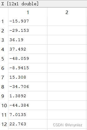
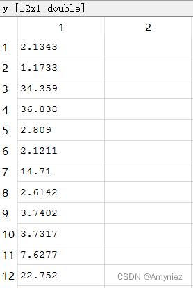
训练集：X、y（12*1）

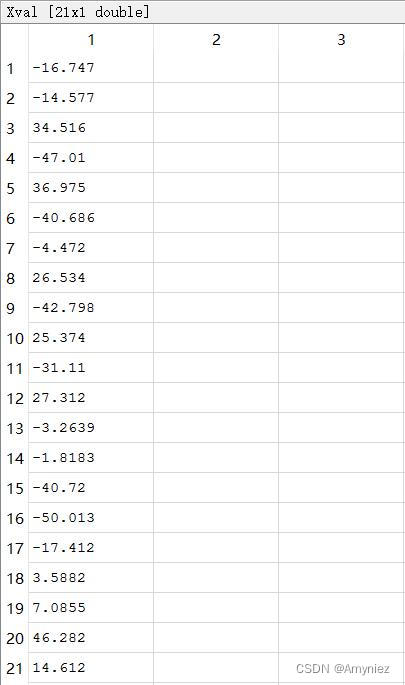
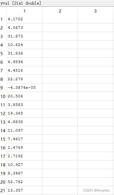
交叉验证集：Xval、yval（21*1）

测试集：Xtest、ytest（21*1）

3. 主程序

%% Initialization
clear ; close all; clc

%% =========== Part 1: Loading and Visualizing Data =============

% Load Training Data
fprintf('Loading and Visualizing Data ...\n')

% You will have X, y, Xval, yval, Xtest, ytest in your environment
load ('ex5data1.mat');

% m是样本个数
m = size(X, 1);

% 绘制训练集train set
plot(X, y, 'rx', 'MarkerSize', 10, 'LineWidth', 1.5);
xlabel('Change in water level (x)');
ylabel('Water flowing out of the dam (y)');

fprintf('Program paused. Press enter to continue.\n');
pause;

%% =========== Part 2: Regularized Linear Regression Cost =============

% 初始化theta
theta = [1 ; 1];
J = linearRegCostFunction([ones(m, 1) X], y, theta, 1);

fprintf(['Cost at theta = [1 ; 1]: %f '], J);

fprintf('Program paused. Press enter to continue.\n');
pause;

%% =========== Part 3: Regularized Linear Regression Gradient =============

theta = [1 ; 1];
% X矩阵前插入一列1，使得X：12*1---> X:12*2
[J, grad] = linearRegCostFunction([ones(m, 1) X], y, theta, 1);

fprintf(['Gradient at theta = [1 ; 1]:  [%f; %f] '], grad(1), grad(2));

fprintf('Program paused. Press enter to continue.\n');
pause;


%% =========== Part 4: Train Linear Regression =============
%  Write Up Note: The data is non-linear, so this will not give a great fit.

%  Train linear regression with lambda = 0
lambda = 0;
[theta] = trainLinearReg([ones(m, 1) X], y, lambda);

%  Plot fit over the data
plot(X, y, 'rx', 'MarkerSize', 10, 'LineWidth', 1.5);
xlabel('Change in water level (x)');
ylabel('Water flowing out of the dam (y)');
hold on;
plot(X, [ones(m, 1) X]*theta, '--', 'LineWidth', 2)
hold off;

fprintf('Program paused. Press enter to continue.\n');
pause;


%% =========== Part 5: Learning Curve for Linear Regression =============

lambda = 0;
[error_train, error_val] = ...
    learningCurve([ones(m, 1) X], y, ...
                  [ones(size(Xval, 1), 1) Xval], yval, ...
                  lambda);

plot(1:m, error_train, 1:m, error_val);
title('Learning curve for linear regression')
legend('Train', 'Cross Validation')
xlabel('Number of training examples')
ylabel('Error')
axis([0 13 0 150])

fprintf('# Training Examples\tTrain Error\tCross Validation Error\n');
for i = 1:m
    fprintf('  \t%d\t\t%f\t%f\n', i, error_train(i), error_val(i));
end

fprintf('Program paused. Press enter to continue.\n');
pause;

%% =========== Part 6: Feature Mapping for Polynomial Regression =============
%  One solution to this is to use polynomial regression.
%  Complete polyFeatures to map each example into its powers
%

p = 8;

% Map X onto Polynomial Features and Normalize
X_poly = polyFeatures(X, p);
[X_poly, mu, sigma] = featureNormalize(X_poly);  % Normalize
X_poly = [ones(m, 1), X_poly];                   % Add Ones

% Map X_poly_test and normalize (using mu and sigma)
X_poly_test = polyFeatures(Xtest, p);
X_poly_test = bsxfun(@minus, X_poly_test, mu);
X_poly_test = bsxfun(@rdivide, X_poly_test, sigma);
X_poly_test = [ones(size(X_poly_test, 1), 1), X_poly_test];         % Add Ones

% Map X_poly_val and normalize (using mu and sigma)
X_poly_val = polyFeatures(Xval, p);
X_poly_val = bsxfun(@minus, X_poly_val, mu);
X_poly_val = bsxfun(@rdivide, X_poly_val, sigma);
X_poly_val = [ones(size(X_poly_val, 1), 1), X_poly_val];           % Add Ones

fprintf('Normalized Training Example 1:\n');
fprintf('  %f  \n', X_poly(1, :));

fprintf('\nProgram paused. Press enter to continue.\n');
pause;



%% =========== Part 7: Learning Curve for Polynomial Regression =============
%  Now, you will get to experiment with polynomial regression with multiple
%  values of lambda. The code below runs polynomial regression with
%  lambda = 0. You should try running the code with different values of
%  lambda to see how the fit and learning curve change.
%

lambda = 0;
[theta] = trainLinearReg(X_poly, y, lambda);

% Plot training data and fit
figure(1);
plot(X, y, 'rx', 'MarkerSize', 10, 'LineWidth', 1.5);
plotFit(min(X), max(X), mu, sigma, theta, p);
xlabel('Change in water level (x)');
ylabel('Water flowing out of the dam (y)');
title (sprintf('Polynomial Regression Fit (lambda = %f)', lambda));

figure(2);
[error_train, error_val] = ...
    learningCurve(X_poly, y, X_poly_val, yval, lambda);
plot(1:m, error_train, 1:m, error_val);

title(sprintf('Polynomial Regression Learning Curve (lambda = %f)', lambda));
xlabel('Number of training examples')
ylabel('Error')
axis([0 13 0 100])
legend('Train', 'Cross Validation')

fprintf('Polynomial Regression (lambda = %f)\n\n', lambda);
fprintf('# Training Examples\tTrain Error\tCross Validation Error\n');
for i = 1:m
    fprintf('  \t%d\t\t%f\t%f\n', i, error_train(i), error_val(i));
end

fprintf('Program paused. Press enter to continue.\n');
pause;

%% =========== Part 8: Validation for Selecting Lambda =============
%  You will now implement validationCurve to test various values of
%  lambda on a validation set. You will then use this to select the
%  "best" lambda value.
%

[lambda_vec, error_train, error_val] = ...
    validationCurve(X_poly, y, X_poly_val, yval);

close all;
plot(lambda_vec, error_train, lambda_vec, error_val);
legend('Train', 'Cross Validation');
xlabel('lambda');
ylabel('Error');

fprintf('lambda\t\tTrain Error\tValidation Error\n');
for i = 1:length(lambda_vec)
	fprintf(' %f\t%f\t%f\n', ...
            lambda_vec(i), error_train(i), error_val(i));
end

fprintf('Program paused. Press enter to continue.\n');
pause;

4.函数实现

4.1 正则化的线性回归的代价函数（linearRegCostFunction）

function [J, grad] = linearRegCostFunction(X, y, theta, lambda)
%LINEARREGCOSTFUNCTION Compute cost and gradient for regularized linear
%regression with multiple variables
%   [J, grad] = LINEARREGCOSTFUNCTION(X, y, theta, lambda) computes the
%   cost of using theta as the parameter for linear regression to fit the
%   data points in X and y. Returns the cost in J and the gradient in grad

% Initialize some useful values
m = length(y); % number of training examples

% You need to return the following variables correctly
J = 0;
grad = zeros(size(theta));

% =================================================================

% 正则化代价函数计算
hypo = X * theta;  % 12*1
Vect_Err = (1/2) .* (hypo-y) .^ 2;
reg = (1/2) .* theta(2:end) .^ 2;
J = (1/m) * (sum(Vect_Err) + lambda * sum(reg));

% 正则化线性回归梯度计算
grad = X' * (hypo - y);
grad_reg = grad(2:end) + lambda .* theta(2:end);
grad = (1/m)*[grad(1); grad_reg];

% =========================================================================

grad = grad(:);

end

4.2 学习曲线（learningCurve）：训练集误差、交叉训练误差

function [error_train, error_val] = ...
    learningCurve(X, y, Xval, yval, lambda)
%LEARNINGCURVE Generates the train and cross validation set errors needed
%to plot a learning curve
%   [error_train, error_val] = ...
%       LEARNINGCURVE(X, y, Xval, yval, lambda) returns the train and
%       cross validation set errors for a learning curve. In particular,
%       it returns two vectors of the same length - error_train and
%       error_val. Then, error_train(i) contains the training error for
%       i examples (and similarly for error_val(i)).
%
%   In this function, you will compute the train and test errors for
%   dataset sizes from 1 up to m. In practice, when working with larger
%   datasets, you might want to do this in larger intervals.
%

% Number of training examples
m = size(X, 1); % 12

% You need to return these values correctly
error_train = zeros(m, 1); % 12*1
error_val   = zeros(m, 1); % 12*1

% =============================================================
% Note: If you are using your cost function (linearRegCostFunction)
%       to compute the training and cross validation error, you should
%       call the function with the lambda argument set to 0.
%       Do note that you will still need to use lambda when running
%       the training to obtain the theta parameters.


for i =1:m,
  % 首先，取样本集中的第一个样本，带入trainLinearReg函数中，该函数会迭代200次，再给出一个关于
  % 样本1的最优theta
  theta = trainLinearReg(X(1:i, :), y(1:i, :), lambda);

  % 然后，利用linearRegCostFunction函数，并设置lambda为0，计算最优theta
  % 在不包含正则项的情况下，样本1的代价函数值error_train(1)
  [error_train(i) grad_train] = linearRegCostFunction(X(1:i, :), y(1:i, :),
  theta, 0);

  % 最后，利用linearRegCostFunction函数，并设置lambda为0，计算最优theta
  % 在不包含正则项的情况下，cross validation set的代价函数值error_val(1)
  [error_val(i) grad_val] = linearRegCostFunction(Xval, yval, theta, 0);
end
% 第二次循环，样本集的样本增加一个，新的样本集包含样本1和样本2


% =========================================================================

end

4.3 特征集变换（polyFeatures）：扩展特征向量到更高维度

function [X_poly] = polyFeatures(X, p)
%POLYFEATURES Maps X (1D vector) into the p-th power
%   [X_poly] = POLYFEATURES(X, p) takes a data matrix X (size m x 1) and
%   maps each example into its polynomial features where
%   X_poly(i, :) = [X(i) X(i).^2 X(i).^3 ...  X(i).^p];
%


for i = 1:p,
  X_poly(:,i) = X .^ i;
end

end

4.4 交叉曲线（validationCurve）

function [lambda_vec, error_train, error_val] = ...
    validationCurve(X, y, Xval, yval)
%VALIDATIONCURVE Generate the train and validation errors needed to
%plot a validation curve that we can use to select lambda
%   [lambda_vec, error_train, error_val] = ...
%       VALIDATIONCURVE(X, y, Xval, yval) returns the train
%       and validation errors (in error_train, error_val)
%       for different values of lambda. You are given the training set (X,
%       y) and validation set (Xval, yval).
%

% Selected values of lambda (you should not change this)
lambda_vec = [0 0.001 0.003 0.01 0.03 0.1 0.3 1 3 10]';


% Instructions: This function to return training errors in
%               error_train and the validation errors in error_val. The
%               vector lambda_vec contains the different lambda parameters
%               to use for each calculation of the errors, i.e,
%               error_train(i), and error_val(i) should give
%               you the errors obtained after training with
%               lambda = lambda_vec(i)
%


for i =1:length(lambda_vec),
  lambda = lambda_vec(i);
  [theta] = trainLinearReg(X,y,lambda);
  error_train(i) = linearRegCostFunction(X,y,theta,0);
  error_val(i) = linearRegCostFunction(Xval,yval,theta,0);
end

end

4.5 特征归一化（featureNormalize）

function [X_norm, mu, sigma] = featureNormalize(X)
%FEATURENORMALIZE Normalizes the features in X 
%   FEATURENORMALIZE(X) returns a normalized version of X where
%   the mean value of each feature is 0 and the standard deviation
%   is 1. This is often a good preprocessing step to do when
%   working with learning algorithms.

mu = mean(X);
X_norm = bsxfun(@minus, X, mu);

sigma = std(X_norm);
X_norm = bsxfun(@rdivide, X_norm, sigma);


% ============================================================

end

4.6 最小化、最优值（fmincg）（最重要的一个部分）

function [X, fX, i] = fmincg(f, X, options, P1, P2, P3, P4, P5)
% Minimize a continuous differentialble multivariate function. Starting point
% is given by "X" (D by 1), and the function named in the string "f", must
% return a function value and a vector of partial derivatives. The Polack-
% Ribiere flavour of conjugate gradients is used to compute search directions,
% and a line search using quadratic and cubic polynomial approximations and the
% Wolfe-Powell stopping criteria is used together with the slope ratio method
% for guessing initial step sizes. Additionally a bunch of checks are made to
% make sure that exploration is taking place and that extrapolation will not
% be unboundedly large. The "length" gives the length of the run: if it is
% positive, it gives the maximum number of line searches, if negative its
% absolute gives the maximum allowed number of function evaluations. You can
% (optionally) give "length" a second component, which will indicate the
% reduction in function value to be expected in the first line-search (defaults
% to 1.0). The function returns when either its length is up, or if no further
% progress can be made (ie, we are at a minimum, or so close that due to
% numerical problems, we cannot get any closer). If the function terminates
% within a few iterations, it could be an indication that the function value
% and derivatives are not consistent (ie, there may be a bug in the
% implementation of your "f" function). The function returns the found
% solution "X", a vector of function values "fX" indicating the progress made
% and "i" the number of iterations (line searches or function evaluations,
% depending on the sign of "length") used.
%
% Usage: [X, fX, i] = fmincg(f, X, options, P1, P2, P3, P4, P5)
%
% See also: checkgrad 
%
% Copyright (C) 2001 and 2002 by Carl Edward Rasmussen. Date 2002-02-13
%
%
% (C) Copyright 1999, 2000 & 2001, Carl Edward Rasmussen
% 
% Permission is granted for anyone to copy, use, or modify these
% programs and accompanying documents for purposes of research or
% education, provided this copyright notice is retained, and note is
% made of any changes that have been made.
% 
% These programs and documents are distributed without any warranty,
% express or implied.  As the programs were written for research
% purposes only, they have not been tested to the degree that would be
% advisable in any important application.  All use of these programs is
% entirely at the user's own risk.
%
% [ml-class] Changes Made:
% 1) Function name and argument specifications
% 2) Output display
%

% Read options
if exist('options', 'var') && ~isempty(options) && isfield(options, 'MaxIter')
    length = options.MaxIter;
else
    length = 100;
end


RHO = 0.01;                            % a bunch of constants for line searches
SIG = 0.5;       % RHO and SIG are the constants in the Wolfe-Powell conditions
INT = 0.1;    % don't reevaluate within 0.1 of the limit of the current bracket
EXT = 3.0;                    % extrapolate maximum 3 times the current bracket
MAX = 20;                         % max 20 function evaluations per line search
RATIO = 100;                                      % maximum allowed slope ratio

argstr = ['feval(f, X'];                      % compose string used to call function
for i = 1:(nargin - 3)
  argstr = [argstr, ',P', int2str(i)];
end
argstr = [argstr, ')'];

if max(size(length)) == 2, red=length(2); length=length(1); else red=1; end
S=['Iteration '];

i = 0;                                            % zero the run length counter
ls_failed = 0;                             % no previous line search has failed
fX = [];
[f1 df1] = eval(argstr);                      % get function value and gradient
i = i + (length<0);                                            % count epochs?!
s = -df1;                                        % search direction is steepest
d1 = -s'*s;                                                 % this is the slope
z1 = red/(1-d1);                                  % initial step is red/(|s|+1)

while i < abs(length)                                      % while not finished
  i = i + (length>0);                                      % count iterations?!

  X0 = X; f0 = f1; df0 = df1;                   % make a copy of current values
  X = X + z1*s;                                             % begin line search
  [f2 df2] = eval(argstr);
  i = i + (length<0);                                          % count epochs?!
  d2 = df2'*s;
  f3 = f1; d3 = d1; z3 = -z1;             % initialize point 3 equal to point 1
  if length>0, M = MAX; else M = min(MAX, -length-i); end
  success = 0; limit = -1;                     % initialize quanteties
  while 1
    while ((f2 > f1+z1*RHO*d1) || (d2 > -SIG*d1)) && (M > 0) 
      limit = z1;                                         % tighten the bracket
      if f2 > f1
        z2 = z3 - (0.5*d3*z3*z3)/(d3*z3+f2-f3);                 % quadratic fit
      else
        A = 6*(f2-f3)/z3+3*(d2+d3);                                 % cubic fit
        B = 3*(f3-f2)-z3*(d3+2*d2);
        z2 = (sqrt(B*B-A*d2*z3*z3)-B)/A;       % numerical error possible - ok!
      end
      if isnan(z2) || isinf(z2)
        z2 = z3/2;                  % if we had a numerical problem then bisect
      end
      z2 = max(min(z2, INT*z3),(1-INT)*z3);  % don't accept too close to limits
      z1 = z1 + z2;                                           % update the step
      X = X + z2*s;
      [f2 df2] = eval(argstr);
      M = M - 1; i = i + (length<0);                           % count epochs?!
      d2 = df2'*s;
      z3 = z3-z2;                    % z3 is now relative to the location of z2
    end
    if f2 > f1+z1*RHO*d1 || d2 > -SIG*d1
      break;                                                % this is a failure
    elseif d2 > SIG*d1
      success = 1; break;                                             % success
    elseif M == 0
      break;                                                          % failure
    end
    A = 6*(f2-f3)/z3+3*(d2+d3);                      % make cubic extrapolation
    B = 3*(f3-f2)-z3*(d3+2*d2);
    z2 = -d2*z3*z3/(B+sqrt(B*B-A*d2*z3*z3));        % num. error possible - ok!
    if ~isreal(z2) || isnan(z2) || isinf(z2) || z2 < 0 % num prob or wrong sign?
      if limit < -0.5                               % if we have no upper limit
        z2 = z1 * (EXT-1);                 % the extrapolate the maximum amount
      else
        z2 = (limit-z1)/2;                                   % otherwise bisect
      end
    elseif (limit > -0.5) && (z2+z1 > limit)         % extraplation beyond max?
      z2 = (limit-z1)/2;                                               % bisect
    elseif (limit < -0.5) && (z2+z1 > z1*EXT)       % extrapolation beyond limit
      z2 = z1*(EXT-1.0);                           % set to extrapolation limit
    elseif z2 < -z3*INT
      z2 = -z3*INT;
    elseif (limit > -0.5) && (z2 < (limit-z1)*(1.0-INT))  % too close to limit?
      z2 = (limit-z1)*(1.0-INT);
    end
    f3 = f2; d3 = d2; z3 = -z2;                  % set point 3 equal to point 2
    z1 = z1 + z2; X = X + z2*s;                      % update current estimates
    [f2 df2] = eval(argstr);
    M = M - 1; i = i + (length<0);                             % count epochs?!
    d2 = df2'*s;
  end                                                      % end of line search

  if success                                         % if line search succeeded
    f1 = f2; fX = [fX' f1]';
    fprintf('%s %4i | Cost: %4.6e\r', S, i, f1);
    s = (df2'*df2-df1'*df2)/(df1'*df1)*s - df2;      % Polack-Ribiere direction
    tmp = df1; df1 = df2; df2 = tmp;                         % swap derivatives
    d2 = df1'*s;
    if d2 > 0                                      % new slope must be negative
      s = -df1;                              % otherwise use steepest direction
      d2 = -s'*s;    
    end
    z1 = z1 * min(RATIO, d1/(d2-realmin));          % slope ratio but max RATIO
    d1 = d2;
    ls_failed = 0;                              % this line search did not fail
  else
    X = X0; f1 = f0; df1 = df0;  % restore point from before failed line search
    if ls_failed || i > abs(length)          % line search failed twice in a row
      break;                             % or we ran out of time, so we give up
    end
    tmp = df1; df1 = df2; df2 = tmp;                         % swap derivatives
    s = -df1;                                                    % try steepest
    d1 = -s'*s;
    z1 = 1/(1-d1);                     
    ls_failed = 1;                                    % this line search failed
  end
  if exist('OCTAVE_VERSION')
    fflush(stdout);
  end
end
fprintf('\n');

4.7 拟合曲线绘制函数（plotFit）

function plotFit(min_x, max_x, mu, sigma, theta, p)
%PLOTFIT Plots a learned polynomial regression fit over an existing figure.
%Also works with linear regression.
%   PLOTFIT(min_x, max_x, mu, sigma, theta, p) plots the learned polynomial
%   fit with power p and feature normalization (mu, sigma).

% Hold on to the current figure
hold on;

% We plot a range slightly bigger than the min and max values to get
% an idea of how the fit will vary outside the range of the data points
x = (min_x - 15: 0.05 : max_x + 25)';

% Map the X values 
X_poly = polyFeatures(x, p);
X_poly = bsxfun(@minus, X_poly, mu);
X_poly = bsxfun(@rdivide, X_poly, sigma);

% Add ones
X_poly = [ones(size(x, 1), 1) X_poly];

% Plot
plot(x, X_poly * theta, '--', 'LineWidth', 2)

% Hold off to the current figure
hold off

end

4.8 训练正则化的线性回归函数（trainLinearReg）

function [theta] = trainLinearReg(X, y, lambda)
%TRAINLINEARREG Trains linear regression given a dataset (X, y) and a
%regularization parameter lambda
%   [theta] = TRAINLINEARREG (X, y, lambda) trains linear regression using
%   the dataset (X, y) and regularization parameter lambda. Returns the
%   trained parameters theta.
%

% Initialize Theta
initial_theta = zeros(size(X, 2), 1); 

% Create "short hand" for the cost function to be minimized
costFunction = @(t) linearRegCostFunction(X, y, t, lambda);

% Now, costFunction is a function that takes in only one argument
options = optimset('MaxIter', 200, 'GradObj', 'on');

% Minimize using fmincg
theta = fmincg(costFunction, initial_theta, options);

end