（2-2）A*算法：A*算法的核心思想

2.2  A*算法的核心思想

A*算法的核心思想是结合实际代价和启发式估计，以高效地搜索图形中的最优路径。通过在评估函数中权衡实际代价和启发式估计，A*算法能够在保证找到最优路径的同时，尽可能减小搜索的时间和空间开销。这使得A*算法成为解决路径规划问题的一种高效而灵活的算法。

2.2.1  A*算法的原理和实现步骤

A*算法的独特之处在于使用启发式估计来引导搜索，从而减少搜索空间，提高效率。A*算法的原理如下所示。

1. 启发式搜索：A*算法是一种启发式搜索算法，利用启发式估计（heuristic estimation）来引导搜索过程。启发式函数h(n)用于估计从当前节点n到目标节点的代价。
2. 综合实际代价和估计代价：A算法综合考虑两个代价：实际代价g(n)，表示从起点到当前节点的实际路径代价，和估计代价h(n)，表示从当前节点到目标节点的启发式估计路径代价。A使用评估函数f(n) = g(n) + h(n) 来确定搜索的优先级。
3. 优先级队列：A*使用一个开放列表（Open List）来存储待考察的节点，按照评估函数f(n)值的优先级排列。在每一步中，选择开放列表中具有最小f(n)值的节点进行探索。
4. 避免重复搜索：通过维护一个关闭列表（Closed List）来避免对已经考察过的节点进行重复搜索，确保算法不会陷入无限循环。

A*算法的实现步骤如下所示。

（1）初始化：将起点加入开放列表（Open List），将关闭列表（Closed List）置为空。

（2）循环直到找到最优路径或开放列表为空：

1. 从开放列表中选择具有最小评估函数f(n)值的节点作为当前节点，将当前节点移到关闭列表。
2. 如果当前节点是目标节点，则路径已找到，进行路径追踪。否则，探索当前节点的邻近节点。

（3）探索邻近节点的，对于当前节点的每个邻近节点：

1. 如果邻近节点在关闭列表中，忽略它。
2. 如果邻近节点不在开放列表中，将其加入开放列表，计算g(n)、h(n)和f(n)值，并设置当前节点为其父节点。
3. 如果邻近节点已经在开放列表中，检查通过当前节点到达邻近节点的路径是否更优，如果是则更新邻近节点的g(n)值和父节点。

（4）路径追踪：当目标节点加入关闭列表，从目标节点沿着父节点一直追溯到起点，构建最短路径。

在实际编程过程中，需要注意以下几点：

1. 数据结构的选择：使用合适的数据结构来表示节点、开放列表和关闭列表，以便高效地进行插入、删除和查找操作。
2. 启发式函数的设计：根据具体问题设计合适的启发式函数，以提高搜索效率。
3. 边界条件的处理：考虑起点和目标点是否可通行，以及处理可能的边界情况。

请看下面的实例，通过A*算法寻找一个6*6网格中给定起点到终点的最短路径。用户输入起点和终点的坐标，然后使用A*算法计算最短路径并在控制台输出路径信息。

实例2-1：使用A*算法计算最短路径（codes/2/easy.py）

实例文件easy.py的具体实现代码如下所示。

import heapq
import numpy as np
import matplotlib.pyplot as plt

class Node:
    def __init__(self, x, y, parent=None, g=0, h=0):
        self.x = x
        self.y = y
        self.parent = parent
        self.g = g
        self.h = h

    def f(self):
        return self.g + self.h
    
    def __lt__(self, other):
        return self.f() < other.f()

def heuristic(node, goal):
    return abs(node.x - goal.x) + abs(node.y - goal.y)

def astar(start, goal, grid):
    open_list = []
    closed_set = set()

    heapq.heappush(open_list, start)
    
    while open_list:
        current_node = heapq.heappop(open_list)

        if current_node.x == goal.x and current_node.y == goal.y:
            path = []
            while current_node:
                path.append((current_node.x, current_node.y))
                current_node = current_node.parent
            return path[::-1]
        
        closed_set.add((current_node.x, current_node.y))

        for dx, dy in [(1, 0), (-1, 0), (0, 1), (0, -1)]:
            new_x, new_y = current_node.x + dx, current_node.y + dy

            if 0 <= new_x < len(grid) and 0 <= new_y < len(grid[0]) and grid[new_x][new_y] == 0 and (new_x, new_y) not in closed_set:
                new_node = Node(new_x, new_y, current_node, current_node.g + 1, heuristic(Node(new_x, new_y), goal))
                heapq.heappush(open_list, new_node)

    return None

def visualize_path(grid, path):
    grid = np.array(grid)
    for x, y in path:
        grid[x][y] = 2
    plt.imshow(grid, cmap='viridis', interpolation='nearest')
    plt.title('Shortest Path')
    plt.show()

def main():
    grid = [
        [0, 0, 0, 0, 0, 0],
        [0, 1, 1, 1, 1, 0],
        [0, 0, 0, 0, 0, 0],
        [0, 1, 1, 1, 1, 0],
        [0, 0, 0, 0, 0, 0],
        [0, 0, 0, 0, 0, 0]
    ]
    start_x, start_y = map(int, input("Enter start coordinates (x y): ").split())
    goal_x, goal_y = map(int, input("Enter goal coordinates (x y): ").split())

    start_node = Node(start_x, start_y)
    goal_node = Node(goal_x, goal_y)

    path = astar(start_node, goal_node, grid)
    if path:
        print("Shortest Path:", path)
        visualize_path(grid, path)
    else:
        print("No path found.")

if __name__ == "__main__":
    main()

上述代码中实现了一个基本的 A* 算法路径规划，并能在给定的迷宫中找到起点到终点的最优路径。上述代码的实现流程如下所示：

（1）首先，定义了一个Node类来表示网格中的节点。每个节点包括其坐标、父节点、从起点到该节点的实际代价（g值）和该节点到目标节点的估计代价（h值）。

（2）然后，实现了启发式函数heuristic，它根据节点与目标节点之间的曼哈顿距离来估计两者之间的距离。

（3）接下来，定义了A*算法函数astar。在这个函数中，使用优先队列（堆）来管理开放列表，并使用集合来管理闭合列表。我们从起点开始，每次选择开放列表中f值（g值加上h值）最小的节点进行扩展。对于每个节点检查其相邻的可行节点，并计算它们的f值。然后，将这些节点加入开放列表，并更新它们的父节点和g值。当找到目标节点或者开放列表为空时，算法终止。

（4）最后，实现了visualize_path函数来可视化找到的路径。这个函数将网格和路径作为输入，并在网格上绘制出路径，最后展示可视化结果。

总体而言，这段代码实现了 A* 算法在给定迷宫中进行路径规划的功能，找到了起点到终点的最短路径，并将其在迷宫中可视化。执行后会打印输出下面的结果，并绘制如图2-8所示的路径可视化图。

Enter start coordinates (x y): 1 1
Enter goal coordinates (x y): 4 4
Shortest Path: [(1, 1), (2, 1), (2, 2), (2, 3), (2, 4), (2, 5), (3, 5), (4, 5), (4, 4)]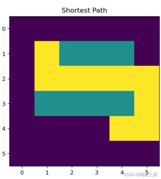

图2-8  路径可视化图

2.2.2  选择启发式函数（估算函数）

选择适当的启发式函数对A*算法的性能至关重要，启发式函数（heuristic function）用于估计从当前节点到目标节点的代价，以指导搜索过程。合理的启发式函数应该在尽量短的时间内提供较为准确的路径代价估计。下面列出了选择启发式函数时的一些常见策略。

（1）曼哈顿距离（Manhattan Distance）

1. 适用于方格网格图形。
2. 计算当前节点到目标节点的水平和垂直距离之和。
3. 在城市街区网格中常用，但不适用于对角线移动。

（2）欧几里得距离（Euclidean Distance）

1. 适用于连续空间的图形。
2. 计算当前节点到目标节点的直线距离。
3. 可能导致在方格网格上过于乐观的估计。

（3）对角线距离

1. 考虑对角线移动，是曼哈顿距离和欧几里得距离的一种折中。
2. 计算水平、垂直和对角线距离的权衡值。

（4）最大方向距离

1. 在方格网格中，计算水平和垂直距离中较大的一个。
2. 避免了对角线移动的过于乐观估计。

（5）自定义启发式函数

1. 根据问题的特性设计特定的启发式函数。
2. 可以利用问题的领域知识来提高估计的准确性。

例如下面的例子实现了A*算法，用于在给定的迷宫地图中寻找从起始节点到目标节点的最短路径，通过使用优先队列和启发式函数（曼哈顿距离）遍历邻居节点并选择代价最小的路径。

实例2-2：使用优先队列和曼哈顿距离寻找最小的路径（codes/2/qi.py）

实例文件qi.py的具体实现代码如下所示。

import heapq
import matplotlib.pyplot as plt
import numpy as np

class Node:
    def __init__(self, x, y, parent=None, g=0, h=0):
        self.x = x
        self.y = y
        self.parent = parent
        self.g = g
        self.h = h

    def f(self):
        return self.g + self.h

    def __lt__(self, other):
        return self.f() < other.f()

def heuristic(node, goal):
    return abs(node.x - goal.x) + abs(node.y - goal.y)

def astar(start, goal, maze):
    open_list = []
    closed_set = set()

    heapq.heappush(open_list, start)
    
    while open_list:
        current_node = heapq.heappop(open_list)

        if current_node.x == goal.x and current_node.y == goal.y:
            path = []
            while current_node:
                path.append((current_node.x, current_node.y))
                current_node = current_node.parent
            return path[::-1], True
        
        closed_set.add((current_node.x, current_node.y))

        for dx, dy in [(1, 0), (-1, 0), (0, 1), (0, -1)]:
            new_x, new_y = current_node.x + dx, current_node.y + dy

            if 0 <= new_x < len(maze) and 0 <= new_y < len(maze[0]) and maze[new_x][new_y] == 0 and (new_x, new_y) not in closed_set:
                new_node = Node(new_x, new_y, current_node, current_node.g + 1, heuristic(Node(new_x, new_y), goal))
                heapq.heappush(open_list, new_node)

    return [], False

def visualize_path(maze, path):
    maze = np.array(maze)
    for x, y in path:
        maze[x][y] = 2
    plt.imshow(maze, cmap='viridis', interpolation='nearest')
    plt.title('Shortest Path')
    plt.show()

def main():
    maze = [
        [0, 0, 1, 0, 0, 0],
        [0, 0, 1, 0, 0, 0],
        [0, 0, 0, 0, 1, 0],
        [0, 0, 1, 1, 1, 0],
        [0, 0, 0, 0, 0, 0]
    ]

    start_x, start_y = 0, 0
    goal_x, goal_y = 4, 5

    start_node = Node(start_x, start_y)
    goal_node = Node(goal_x, goal_y)

    path, found = astar(start_node, goal_node, maze)
    if found:
        print("Shortest Path:", path)
        visualize_path(maze, path)
    else:
        print("No path found.")

if __name__ == "__main__":
    main()

在上述代码中，使用优先队列来管理开放列表，并且使用了启发式函数来估计节点之间的距离。在A*算法的实现中，函数heappush和函数heappop使用了优先队列来确保每次从开放列表中取出的节点都是具有最小代价的节点。同时，函数heuristic计算了节点之间的曼哈顿距离作为启发式函数，用于估计节点之间的实际代价。执行后会打印输出如下找到的最短路径，并绘制如图2-8所示的路径可视化图。

Shortest Path: [(0, 0), (1, 0), (2, 0), (3, 0), (3, 1), (4, 1), (4, 2), (4, 3), (4, 4), (4, 5)]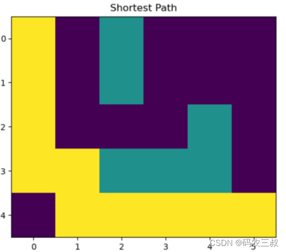

图2-8  路径可视化图

注意：在选择启发式函数时，需要权衡准确性和计算效率。过于简单的启发式函数可能导致算法收敛速度慢，而过于复杂的函数可能使算法变得过于计算密集。在实践应用中，不同问题可能需要尝试不同的启发式函数，以找到最适合问题特性的估计方法。