Automatic Differentiation Part 1

最新推荐文章于 2024-08-24 14:08:21 发布

张博208

最新推荐文章于 2024-08-24 14:08:21 发布

阅读量829

点赞数 14

分类专栏： Machine Learning 文章标签：算法

本文链接：https://blog.csdn.net/bbbeoy/article/details/139376056

版权

Machine Learning 专栏收录该内容

208 篇文章 14 订阅

订阅专栏

Automatic Differentiation Part 1: Understanding the Math

In this tutorial, you will learn the math behind automatic differentiation needed for backpropagation.

Automatic Differentiation Part 1: Understanding the Math

Imagine you are trekking down a hill. It is dark, and there are a lot of bumps and turns. You have no way of knowing how to reach the center. Now imagine every time you progress, you have to pause, take out the topological map of the hill and calculate your direction and speed for the next set. Sounds painfully less fun, right?

If you have been a reader of our tutorials, you would know what that analogy refers to. The hill is your loss landscape, the topological map is the set of rules for multivariate calculus, and you are the parameters of the neural network. The objective is to reach the global minimum.

And that brings us to the question:

Why do we use a Deep Learning Framework today?

The first thing that pops into the mind is automatic differentiation. We write the forward pass, and that is it; no need to worry about the backward pass. Every operator is automatically differentiated and is waiting to be used in an optimization algorithm (like stochastic gradient descent).

Today in this tutorial, we will walk through the valleys of automatic differentiation.

Introduction

In this section, we will lay out the foundation necessary for understanding

autodiff

Jacobian

Let’s consider a function

$F \colon \mathbb{R}^{n} \to \mathbb{R}$

is a multivariate function that simultaneously depends on multiple variables. Here the multiple variables can be

$x = \{x_{1}, x_{2}, \ldots, x_{n}\}$

. The output of the function is a scalar value. This can be considered as a neural network that takes an image and outputs the probability of a dog’s presence in the image.

Note: Let us recall that in a neural network, we compute gradients with respect to the parameters (weights and biases) and not the inputs (the image). Thus the domain of the function is the parameters and not the inputs, which helps keep the gradient computation accessible. We need to now think of everything we do in this tutorial from the perspective of making it simple and efficient to obtain the gradients with respect to the weights and biases (parameters). This is illustrated in Figure 1.

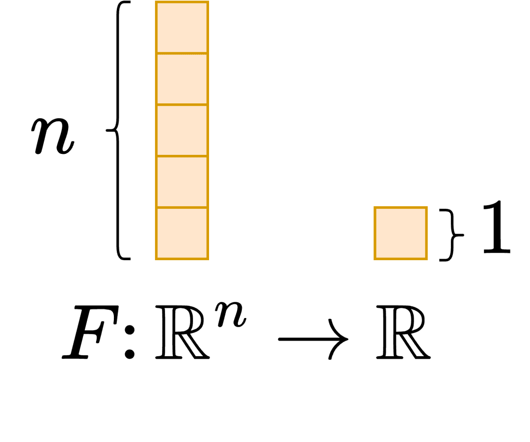
Figure 1: Domain of the function from the perspective of a neural network (source: image by the authors).

A neural network is a composition of many sublayers. So let’s consider our function

as a composition of multiple functions (primitive operations).

$F(x) \ = \ D \circ C \circ B \circ A$

The function

is composed of four primitive functions, namely

$D, C, B, \text{ and } A$

. For anyone new to composition, we can call

to be a function where

is equal to

The next step would be to find the gradient of

. However, before diving into the gradients of the function, let us revisit Jacobian matrices. It turns out that the derivatives of a multivariate function are a Jacobian matrix consisting of partial derivatives of the function w.r.t. all the variables upon which it depends.

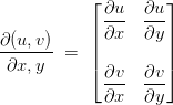
Consider two multivariate functions,

and

, which depend on the variables

and

. The Jacobian would look like this:

$\displaystyle\frac{\partial{(u, v)}}{\partial{x, y}} \ = \ \begin{bmatrix} \displaystyle\frac{\partial u}{\partial x} & \displaystyle\frac{\partial u}{\partial y}\\ \\ \displaystyle\frac{\partial v}{\partial x} & \displaystyle\frac{\partial v}{\partial y} \end{bmatrix}$

Now let’s compute the Jacobian of our function

. We need to note here that the function depends of

variables

$x = \{x_{1}, x_{2}, \ldots, x_{n}\}$

, and outputs a scalar value. This means that the Jacobian will be a row vector.

$F^\prime(x) \ = \ \displaystyle\frac{\partial{y}}{\partial{x}} \ = \ \begin{bmatrix} \displaystyle\frac{\partial y}{\partial x_{1}} & \ldots & \displaystyle\frac{\partial y}{\partial x_{n}} \end{bmatrix}$

Chain Rule

Remember how our function

is composed of many primitive functions? The derivative of such a composed function is done with the help of the chain rule. To help our way into the chain rule, let us first write down the composition and then define the intermediate values.

is composed of:

Now that the composition is spelled out, let’s first get the derivatives of the intermediate values.

$D^\prime(c) = \displaystyle\frac{\partial{y}}{\partial{c}}$
$C^\prime(b) = \displaystyle\frac{\partial{c}}{\partial{b}}$
$B^\prime(a) = \displaystyle\frac{\partial{b}}{\partial{a}}$
$A^\prime(x) = \displaystyle\frac{\partial{a}}{\partial{x}}$

Now with the help of the chain rule, we derive the derivative of the function

$F^\prime(x) \ = \ \displaystyle\frac{\partial{y}}{\partial{c}} \displaystyle\frac{\partial{c}}{\partial{b}} \displaystyle\frac{\partial{b}}{\partial{a}} \displaystyle\frac{\partial{a}}{\partial{x}}$

Mix the Jacobian and Chain Rule

After knowing about the Jacobian and the Chain Rule, let us visualize the two together. Shown in Figure 2.

$F^\prime(x) \ = \ \displaystyle\frac{\partial{y}}{\partial{c}} \displaystyle\frac{\partial{c}}{\partial{b}} \displaystyle\frac{\partial{b}}{\partial{a}} \displaystyle\frac{\partial{a}}{\partial{x}}$

Figure 2: Jacobian and chain rule together (source: image by the authors).

The derivative of our function

is just the matrix multiplication of the Jacobian matrices of the intermediate terms.

Now, this is where we ask the question:

Does it matter the order in which we do the matrix multiplication?

Forward and Reverse Accumulations

In this section, we try to understand the answer to the question of ordering the Jacobian matrix multiplication.

There are two extremes in which we could order the multiplications: the forward accumulation and the reverse accumulation.

Forward Accumulation

If we order the multiplication from right to left in the same order in which the function

was evaluated, the process is called forward accumulation. The best way to think about the ordering is to place brackets in the equation, as shown in Figure 3.

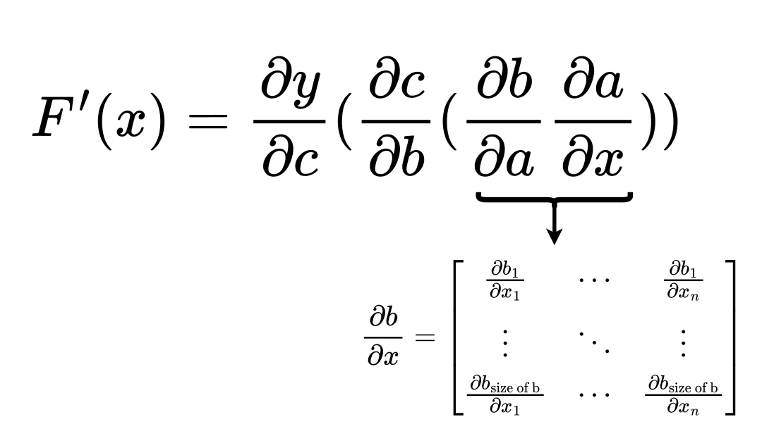
$F^\prime(x) \ = \ \displaystyle\frac{\partial{y}}{\partial{c}} \left(\frac{\partial{c}}{\partial{b}} \left(\frac{\partial{b}}{\partial{a}} \displaystyle\frac{\partial{a}}{\partial{x}}\right)\right)$

Figure 3: Forward accumulation of gradients (source: image by the authors).

With the function

$F : \mathbb{R}^{n} \to \mathbb{R}$

, the forward accumulation process is matrix multiplication in all the steps. This is more FLOPs.

Note: Forward accumulation is beneficial when we want to get the derivative of a function

$F: \mathbb{R} \to \mathbb{R}^{n}$

Another way to understand forwarding accumulation is to think of a Jacobian-Vector Product (JVP). Consider a Jacobian

$F^\prime(x)$

and a vector

. The Jacobian-Vector Product would look to be

$F^\prime(x)v$

$F^\prime(x)v \ = \ \displaystyle\frac{\partial{y}}{\partial{c}} \left(\displaystyle\frac{\partial{c}}{\partial{b}} \left(\displaystyle\frac{\partial{b}}{\partial{a}} \left(\displaystyle\frac{\partial{a}}{\partial{x}} v\right)\right)\right)$

This is done for us to have matrix-vector multiplication at all the stages (which makes the process more efficient).

➤ Question: If we have a Jacobian-Vector Product, how can we obtain the Jacobian from it?

➤ Answer: We pass a one-hot vector and get each column of the Jacobian one at a time.

So we can think of forwarding accumulation as a process in which we build the Jacobian per column.

Reverse Accumulation

Suppose we order the multiplication from left to right, in the opposite direction to which the function was evaluated. In that case, the process is called reverse accumulation. The diagram of the process is illustrated in Figure 4.

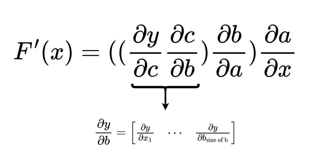
$F^\prime(x) \ = \ \left(\left(\displaystyle\frac{\partial{y}}{\partial{c}} \displaystyle\frac{\partial{c}}{\partial{b}}\right) \displaystyle\frac{\partial{b}}{\partial{a}} \right)\displaystyle\frac{\partial{a}}{\partial{x}}$

Figure 4: Reverse accumulation of gradients (source: image by the authors).

As it turns out, with reverse accumulation deriving the derivative of a function

$F : \mathbb{R}^{n} \to \mathbb{R}$

is a vector to matrix multiplication at all steps. This means that for the particular function, reverse accumulation has lesser FLOPs than forwarding accumulation.

Another way to understand forwarding accumulation is to think of a Vector-Jacobian Product (VJP). Consider a Jacobian

$F^\prime(x)$

and a vector

. The Vector-Jacobian Product would look to be

$v^{T}F^\prime(x)$

$v^{T}F^\prime(x) \ = \ \left(\left(\left(v^{T} \displaystyle\frac{\partial{y}}{\partial{c}}\right) \displaystyle\frac{\partial{c}}{\partial{b}}\right) \displaystyle\frac{\partial{b}}{\partial{a}}\right)\displaystyle\frac{\partial{a}}{\partial{x}}$

This allows us to have vector-matrix multiplication at all stages (which makes the process more efficient).

➤ Question: If we have a Vector-Jacobian Product, how can we obtain the Jacobian from it?

➤ Answer: We pass a one-hot vector and get each row of the Jacobian one at a time.

So we can think of reverse accumulation as a process in which we build the Jacobian per row.

Now, if we consider our previously mentioned function

, we know that the Jacobian

$F^\prime(x)$

is a row vector. Therefore, if we apply the reverse accumulation process, which means the Vector-Jacobian Product, we can obtain the row vector in one shot. On the other hand, if we apply the forward accumulation process, the Jacobian-Vector Product, we will obtain a single element as a column, and we would need to iterate to build the entire row.

This is why reverse accumulation is used more often in the Neural Network literature.

Summary

In this tutorial, we studied the math of automatic differentiation and how it is applied to the parameters of a Neural Network. The next tutorial will expand on this and see how we can implement automatic differentiation using a python package. The implementation will involve a step-by-step walkthrough of creating a python package and using it to train a neural network.

Did you enjoy a math-heavy tutorial on the fundamentals of automatic differentiation? Let us know.