


Automatic Differentiation Part 2: Implementation Using Micrograd
Introduction
What Is a Neural Network?
A Neural Network is a mathematical abstraction of our brain (at least, that is how it all started). The system consists of many learnable knobs (weights and biases) and a simple operation (dot product). The Neural Network takes in inputs and uses an objective function that we need to optimize by turning the knobs. The best way to tune the knobs is to use the gradient of the objective function with respect to all the individual knobs as a signal.
It will take a long time if you sit down and try to calculate the gradient by hand. So, to bypass this process, we use the concept of automatic differentiation.
In the previous tutorial, we deeply studied the mathematics of automatic differentiation. This tutorial will apply the concepts and work our way into understanding an automatic differentiation Python package from scratch.
The package that we will talk about today is called
. This is an open-source Python package created by Andrej Karpathy. We have studied the video lecture, where Andrej built the package from scratch. Here, we break down the video lecture into a blog where we add our thoughts to enrich the content.
About micrograd
micrograd
is a Python package built to understand how the reverse accumulation (backpropagation) process works in a modern deep learning package like PyTorch or Jax. It is a simple automatic differentiation package that works with scalars only.
Imports and Setup
→ Launch Jupyter Notebook on Google Colab → Launch Jupyter Notebook on Google Colab
Automatic Differentiation Part 2: Implementation Using Micrograd
import math
import random
from typing import List, Tuple, Union
from matplotlib import pyplot as plt
The Value Class
We start things off by defining the
Value
class. To work on tracing and backpropagation later, it becomes essential to wrap raw scalar values into the
Value
class.
When wrapped inside the
Value
class, the scalar value is considered a Node of a Graph. When we use
Value
s and build an equation, the equation is considered a Directed Acyclic Graph (DAG). With the help of calculus and graph traversal, we compute the gradients of the nodes automatically (autodiff) and backpropagate through them.
The
Value
class has the following attributes:
-
data
: The raw float data that needs to be wrapped inside theValue
class. -
grad
: This will hold the global derivative of the node. The global derivative is the partial derivative of the root node (final node) with respect to the current node. -
_backward
: This is a private method that computes the global derivative of the children of the current node. -
_prev
: The children of the current node.
→ Launch Jupyter Notebook on Google Colab → Launch Jupyter Notebook on Google Colab
Automatic Differentiation Part 2: Implementation Using Micrograd
class Value(object):
"""
We need to wrap the raw data into a class that will store the
metadata to help in automatic differentiation.
Attributes:
data (float): The data for the Value node.
_children (Tuple): The children of the current node.
"""
def __init__(self, data: float, _children: Tuple = ()):
# The raw data for the Value node.
self.data = data
# The partial gradient of the last node with respect to this
# node. This is also termed as the global gradient.
# Gradient 0.0 means that there is no effect of the change
# of the last node with respect to this node. On
# initialization it is assumed that all the variables have no
# effect on the entire architecture.
self.grad = 0.0
# The function that derives the gradient of the children nodes
# of the current node. It is easier this way, because each node
# is built from children nodes and an operation. Upon back-propagation
# the current node can easily fill in the gradients of the children.
# Note: The global gradient is the multiplication of the local gradient
# and the flowing gradient from the parent.
self._backward = lambda: None
# Define the children of this node.
self._prev = set(_children)
def __repr__(self):
# This is the string representation of the Value node.
return f"Value(data={self.data}, grad={self.grad})"
→ Launch Jupyter Notebook on Google Colab → Launch Jupyter Notebook on Google Colab
Automatic Differentiation Part 2: Implementation Using Micrograd
# Build a Value node
raw_data = 5.0
print(f"Raw Data(data={raw_data}, type={type(raw_data)}")
value_node = Value(data=raw_data)
# Calling the `__repr__` function here
print(value_node)
→ Launch Jupyter Notebook on Google Colab → Launch Jupyter Notebook on Google Colab
Automatic Differentiation Part 2: Implementation Using Micrograd
>>> Raw Data(data=5.0, type=<class 'float'>
>>> Value(data=5.0, grad=0.0)
Addition
Now that we have built our
Value
class, we need to define the primitive operations and their
_backward
functions. This will help trace each node’s operations and back-propagate the gradients through the DAG expression.
In this section, we deal with the addition operation. This will help in two values being added together. Python classes have a special method
__add__
called when we use the
+
operator, as shown in Figure 1.
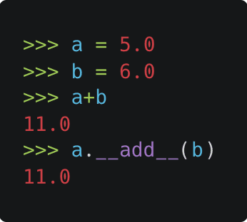
Figure 1:
__add__
dunder function (source: image by the authors).
Here we create the
custom_addition
function that is later assigned to the
__add__
method of the
Value
class. This is done for us to focus on the addition method and discard everything that is not important to the addition operation.
The addition operation is as simple as it gets:
- The
self
and theother
nodes as an argument to the call. We then take theirdata
and apply addition. - The result is then wrapped inside the
Value
class. - The
out
node is initialized, where we mention thatself
andother
are its children.
Compute Gradient
We will have this section for every primitive operation that we define. For example, to compute the global gradient of the children nodes, we need to define the local gradient of the
addition
operation.
Let us consider a node
![]()
that is built by adding two children nodes
![]()
and
![]()
. Then, the partial derivatives of
![]()
are derived in Figure 2.

Figure 2: Local gradient of addition operation (source: image by the authors).
Now think of backpropagation. The partial derivative of the loss (objective) function
![]()
is already deduced for
![]()
. This means we have
![]()
. This gradient needs to flow to the child nodes
![]()
and
![]()
, respectively.
Applying the chain rule, we get the global gradient for
![]()
and
![]()
, as shown in Figure 3.
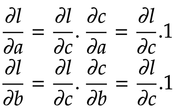
Figure 3: Global derivative of addition operation (source: image by the authors).
The addition operation acts like a router to the gradients flowing in. It routes the gradients to all the children.
➤ Note: In the
_backward
functions that we define, we accumulate the gradients of the children with the
+=
operation. This is done to bypass a unique case. Suppose we have
![]()
. Here we know that the expression can be simplified to
![]()
, but our
_backward
for
__add__
does not know how to do this. The
__backward__
in
__add__
treats one
![]()
as
self
and the other
![]()
as
other
. If the gradients are not accumulated, we will see a discrepancy with the gradients. → Launch Jupyter Notebook on Google Colab → Launch Jupyter Notebook on Google Colab
Automatic Differentiation Part 2: Implementation Using Micrograd
def custom_addition(self, other: Union["Value", float]) -> "Value":
"""
The addition operation for the Value class.
Args:
other (Union["Value", float]): The other value to add to this one.
Usage:
>>> x = Value(2)
>>> y = Value(3)
>>> z = x + y
>>> z.data
5
"""
# If the other value is not a Value, then we need to wrap it.
other = other if isinstance(other, Value) else Value(other)
# Create a new Value node that will be the output of the addition.
out = Value(data=self.data + other.data, _children=(self, other))
def _backward():
# Local gradient:
# x = a + b
# dx/da = 1
# dx/db = 1
# Global gradient with chain rule:
# dy/da = dy/dx . dx/da = dy/dx . 1
# dy/db = dy/dx . dx/db = dy/dx . 1
self.grad += out.grad * 1.0
other.grad += out.grad * 1.0
# Set the backward function on the output node.
out._backward = _backward
return out
def custom_reverse_addition(self, other):
"""
Reverse addition operation for the Value class.
Args:
other (float): The other value to add to this one.
Usage:
>>> x = Value(2)
>>> y = Value(3)
>>> z = y + x
>>> z.data
5
"""
# This is the same as adding. We can reuse the __add__ method.
return self + other
Value.__add__ = custom_addition
Value.__radd__ = custom_reverse_addition
→ Launch Jupyter Notebook on Google Colab → Launch Jupyter Notebook on Google Colab
Automatic Differentiation Part 2: Implementation Using Micrograd
# Build a and b
a = Value(data=5.0)
b = Value(data=6.0)
# Print the addition
print(f"{a} + {b} => {a+b}")
→ Launch Jupyter Notebook on Google Colab → Launch Jupyter Notebook on Google Colab
Automatic Differentiation Part 2: Implementation Using Micrograd
>>> Value(data=5.0, grad=0.0) + Value(data=6.0, grad=0.0) => Value(data=11.0, grad=0.0)
→ Launch Jupyter Notebook on Google Colab → Launch Jupyter Notebook on Google Colab
Automatic Differentiation Part 2: Implementation Using Micrograd
# Add a and b
c = a + b
# Assign a global gradient to c
c.grad = 11.0
print(f"c => {c}")
# Now apply `_backward` to c
c._backward()
print(f"a => {a}")
print(f"b => {b}")
→ Launch Jupyter Notebook on Google Colab → Launch Jupyter Notebook on Google Colab
Automatic Differentiation Part 2: Implementation Using Micrograd
>>> c => Value(data=11.0, grad=11.0)
>>> a => Value(data=5.0, grad=11.0)
>>> b => Value(data=6.0, grad=11.0)
➤ Note: The global gradient of
![]()
is routed to
![]()
and
![]()
.
Multiplication
In this section, we deal with the multiplication operation. Python classes have a special method
__mul__
called when we use the
*
operator, as shown in Figure 4.
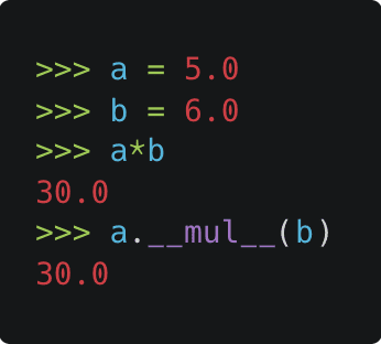
Figure 4:
__mul__
dunder method (source: image by the authors).
We get the
self
and the
other
nodes as an argument to the call. We then take their
data
and apply multiplication. The result is then wrapped inside the
Value
class. Finally, the
out
node is initialized, where we mention that
self
and
other
are its children.
Compute Gradient
Let us consider a node
![]()
that is built by multiplying two children nodes
![]()
and
![]()
. Then, the partial derivatives of
![]()
are shown in Figure 5.
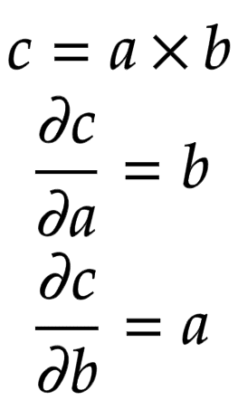
Figure 5: Local gradient of multiplication operation (source: image by the authors).
Now think of backpropagation. The partial derivative of the loss (objective) function
![]()
is already deduced for
![]()
. This means we have
![]()
. This gradient needs to flow to the children nodes
![]()
and
![]()
, respectively.
Applying the chain rule, we get the global gradient for
![]()
and
![]()
, as shown in Figure 6.
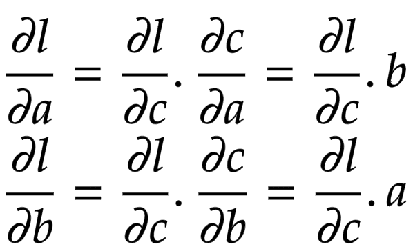
Figure 6: Global gradient of multiplication operation (source: image by the authors).
→ Launch Jupyter Notebook on Google Colab → Launch Jupyter Notebook on Google Colab
Automatic Differentiation Part 2: Implementation Using Micrograd
def custom_multiplication(self, other: Union["Value", float]) -> "Value":
"""
The multiplication operation for the Value class.
Args:
other (float): The other value to multiply to this one.
Usage:
>>> x = Value(2)
>>> y = Value(3)
>>> z = x * y
>>> z.data
6
"""
# If the other value is not a Value, then we need to wrap it.
other = other if isinstance(other, Value) else Value(other)
# Create a new Value node that will be the output of
# the multiplication.
out = Value(data=self.data * other.data, _children=(self, other))
def _backward():
# Local gradient:
# x = a * b
# dx/da = b
# dx/db = a
# Global gradient with chain rule:
# dy/da = dy/dx . dx/da = dy/dx . b
# dy/db = dy/dx . dx/db = dy/dx . a
self.grad += out.grad * other.data
other.grad += out.grad * self.data
# Set the backward function on the output node.
out._backward = _backward
return out
def custom_reverse_multiplication(self, other):
"""
Reverse multiplication operation for the Value class.
Args:
other (float): The other value to multiply to this one.
Usage:
>>> x = Value(2)
>>> y = Value(3)
>>> z = y * x
>>> z.data
6
"""
# This is the same as multiplying. We can reuse the __mul__ method.
return self * other
Value.__mul__ = custom_multiplication
Value.__rmul__ = custom_reverse_multiplication
→ Launch Jupyter Notebook on Google Colab → Launch Jupyter Notebook on Google Colab
Automatic Differentiation Part 2: Implementation Using Micrograd
# Build a and b
a = Value(data=5.0)
b = Value(data=6.0)
# Print the multiplication
print(f"{a} * {b} => {a*b}")
→ Launch Jupyter Notebook on Google Colab → Launch Jupyter Notebook on Google Colab
Automatic Differentiation Part 2: Implementation Using Micrograd
>>> Value(data=5.0, grad=0.0) * Value(data=6.0, grad=0.0) => Value(data=30.0, grad=0.0)
→ Launch Jupyter Notebook on Google Colab → Launch Jupyter Notebook on Google Colab
Automatic Differentiation Part 2: Implementation Using Micrograd
# Multiply a and b
c = a * b
# Assign a global gradient to c
c.grad = 11.0
print(f"c => {c}")
# Now apply `_backward` to c
c._backward()
print(f"a => {a}")
print(f"b => {b}")
→ Launch Jupyter Notebook on Google Colab → Launch Jupyter Notebook on Google Colab
Automatic Differentiation Part 2: Implementation Using Micrograd
>>> c => Value(data=30.0, grad=11.0)
>>> a => Value(data=5.0, grad=66.0)
>>> b => Value(data=6.0, grad=55.0)
Power
In this section, we deal with the power operation. Python classes have a special method
__pow__
that is called when we use the
**
operator, as shown in Figure 7.
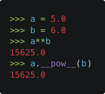
Figure 7:
__pow__
dunder function (source: image by the authors).
After obtaining the
self
and the
other
nodes as an argument to the call, we take their
data
and apply the power operation.
Compute Gradient
Let us consider a node
![]()
that is built by multiplying two children nodes
![]()
and
![]()
. Then, the partial derivatives of
![]()
are derived in Figure 8.
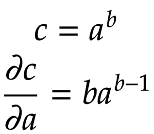
Figure 8: Local gradient of power operation (source: image by the authors).
Now think of backpropagation. The partial derivative of the loss (objective) function
![]()
is already deduced for
![]()
. This means we have
![]()
. This gradient needs to flow to the child node
![]()
.
Applying the chain rule, we get the global gradient for
![]()
and
![]()
, as shown in Figure 9.
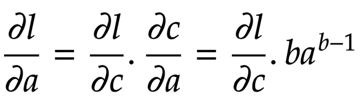
Figure 9: Global gradient of power operation (source: image by the authors).
→ Launch Jupyter Notebook on Google Colab → Launch Jupyter Notebook on Google Colab
Automatic Differentiation Part 2: Implementation Using Micrograd
def custom_power(self, other):
"""
The power operation for the Value class.
Args:
other (float): The other value to raise this one to.
Usage:
>>> x = Value(2)
>>> z = x ** 2.0
>>> z.data
4
"""
assert isinstance(
other, (int, float)
), "only supporting int/float powers for now"
# Create a new Value node that will be the output of the power.
out = Value(data=self.data ** other, _children=(self,))
def _backward():
# Local gradient:
# x = a ** b
# dx/da = b * a ** (b - 1)
# Global gradient:
# dy/da = dy/dx . dx/da = dy/dx . b * a ** (b - 1)
self.grad += out.grad * (other * self.data ** (other - 1))
# Set the backward function on the output node.
out._backward = _backward
return out
Value.__pow__ = custom_power
→ Launch Jupyter Notebook on Google Colab → Launch Jupyter Notebook on Google Colab
Automatic Differentiation Part 2: Implementation Using Micrograd
# Build a
a = Value(data=5.0)
# For power operation we will use
# the raw data and not wrap it into
# a node. This is done for simplicity.
b = 2.0
# Print the power operation
print(f"{a} ** {b} => {a**b}")
→ Launch Jupyter Notebook on Google Colab → Launch Jupyter Notebook on Google Colab
Automatic Differentiation Part 2: Implementation Using Micrograd
>>> Value(data=5.0, grad=0.0) ** 2.0 => Value(data=25.0, grad=0.0)
→ Launch Jupyter Notebook on Google Colab → Launch Jupyter Notebook on Google Colab
Automatic Differentiation Part 2: Implementation Using Micrograd
# Raise a to the power of b
c = a ** b
# Assign a global gradient to c
c.grad = 11.0
print(f"c => {c}")
# Now apply `_backward` to c
c._backward()
print(f"a => {a}")
print(f"b => {b}")
→ Launch Jupyter Notebook on Google Colab → Launch Jupyter Notebook on Google Colab
Automatic Differentiation Part 2: Implementation Using Micrograd
>>> c => Value(data=25.0, grad=11.0)
>>> a => Value(data=5.0, grad=110.0)
>>> b => 2.0
Negation
For the negation operation, we will be using the
__mul__
operation defined above. In addition, Python classes have a special method
__neg__
called when we use the unary
-
operator, as shown in Figure 10.
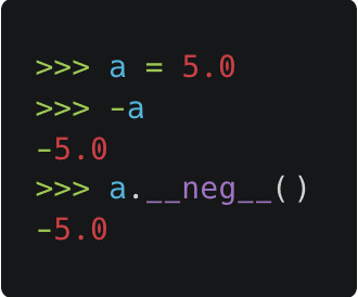
Figure 10:
__neg__
dunder function (source: image by the authors).
This means the
_backward
of negation will be taken care of, and we would not have to define it explicitly. → Launch Jupyter Notebook on Google Colab → Launch Jupyter Notebook on Google Colab
Automatic Differentiation Part 2: Implementation Using Micrograd
def custom_negation(self):
"""
Negation operation for the Value class.
Usage:
>>> x = Value(2)
>>> z = -x
>>> z.data
-2
"""
# This is the same as multiplying by -1. We can reuse the
# __mul__ method.
return self * -1
Value.__neg__ = custom_negation
→ Launch Jupyter Notebook on Google Colab → Launch Jupyter Notebook on Google Colab
Automatic Differentiation Part 2: Implementation Using Micrograd
# Build `a`
a = Value(data=5.0)
# Print the negation
print(f"Negation of {a} => {(-a)}")
→ Launch Jupyter Notebook on Google Colab → Launch Jupyter Notebook on Google Colab
Automatic Differentiation Part 2: Implementation Using Micrograd
>>> Negation of Value(data=5.0, grad=0.0) => Value(data=-5.0, grad=0.0)
→ Launch Jupyter Notebook on Google Colab → Launch Jupyter Notebook on Google Colab
Automatic Differentiation Part 2: Implementation Using Micrograd
# Negate a
c = -a
# Assign a global gradient to c
c.grad = 11.0
print(f"c => {c}")
# Now apply `_backward` to c
c._backward()
print(f"a => {a}")
→ Launch Jupyter Notebook on Google Colab → Launch Jupyter Notebook on Google Colab
Automatic Differentiation Part 2: Implementation Using Micrograd
>>> c => Value(data=-5.0, grad=11.0)
>>> a => Value(data=5.0, grad=-11.0)
Subtraction
The subtraction operation can be handled with
__add__
and
__neg__
. In addition, Python classes have a special method
__sub__
called when we use the
-
operator, as shown in Figure 11.
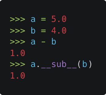
Figure 11:
__sub__
dunder function (source: image by the authors).
This will help us delegate the
_backward
subtraction operation to the addition and negation operations. → Launch Jupyter Notebook on Google Colab → Launch Jupyter Notebook on Google Colab
Automatic Differentiation Part 2: Implementation Using Micrograd
def custom_subtraction(self, other):
"""
Subtraction operation for the Value class.
Args:
other (float): The other value to subtract to this one.
Usage:
>>> x = Value(2)
>>> y = Value(3)
>>> z = x - y
>>> z.data
-1
"""
# This is the same as adding the negative of the other value.
# We can reuse the __add__ and the __neg__ methods.
return self + (-other)
def custom_reverse_subtraction(self, other):
"""
Reverse subtraction operation for the Value class.
Args:
other (float): The other value to subtract to this one.
Usage:
>>> x = Value(2)
>>> y = Value(3)
>>> z = y - x
>>> z.data
1
"""
# This is the same as subtracting. We can reuse the __sub__ method.
return other + (-self)
Value.__sub__ = custom_subtraction
Value.__rsub__ = custom_reverse_subtraction
→ Launch Jupyter Notebook on Google Colab → Launch Jupyter Notebook on Google Colab
Automatic Differentiation Part 2: Implementation Using Micrograd
# Build a and b
a = Value(data=5.0)
b = Value(data=4.0)
# Print the negation
print(f"{a} - {b} => {(a-b)}")
→ Launch Jupyter Notebook on Google Colab → Launch Jupyter Notebook on Google Colab
Automatic Differentiation Part 2: Implementation Using Micrograd
>>> Value(data=5.0, grad=0.0) - Value(data=4.0, grad=0.0) => Value(data=1.0, grad=0.0)
→ Launch Jupyter Notebook on Google Colab → Launch Jupyter Notebook on Google Colab
Automatic Differentiation Part 2: Implementation Using Micrograd
# Subtract b from a
c = a - b
# Assign a global gradient to c
c.grad = 11.0
print(f"c => {c}")
# Now apply `_backward` to c
c._backward()
print(f"a => {a}")
print(f"b => {b}")
→ Launch Jupyter Notebook on Google Colab → Launch Jupyter Notebook on Google Colab
Automatic Differentiation Part 2: Implementation Using Micrograd
>>> c => Value(data=1.0, grad=11.0)
>>> a => Value(data=5.0, grad=11.0)
>>> b => Value(data=4.0, grad=0.0)
➤ Note: The gradients did not flow as they were supposed to on paper. Why? Can you figure out the answer to this?
➤ Hint: The subtraction operation consists of more than one primitive operation: negation and addition.
We will discuss this later in the tutorial.
Division
The division operation can be handled with
__mul__
and
__pow__
. In addition, Python classes have a special method
__div__
called when we use the
/
operator, as shown in Figure 12.

Figure 12:
__div__
dunder function (source: image by the authors).
This will help us delegate the
_backward
division operation to the power operation. → Launch Jupyter Notebook on Google Colab → Launch Jupyter Notebook on Google Colab
Automatic Differentiation Part 2: Implementation Using Micrograd
def custom_division(self, other):
"""
Division operation for the Value class.
Args:
other (float): The other value to divide to this one.
Usage:
>>> x = Value(10)
>>> y = Value(5)
>>> z = x / y
>>> z.data
2
"""
# Use the __pow__ method to implement division.
return self * other ** -1
def custom_reverse_division(self, other):
"""
Reverse division operation for the Value class.
Args:
other (float): The other value to divide to this one.
Usage:
>>> x = Value(10)
>>> y = Value(5)
>>> z = y / x
>>> z.data
0.5
"""
# Use the __pow__ method to implement division.
return other * self ** -1
Value.__truediv__ = custom_division
Value.__rtruediv__ = custom_reverse_division
→ Launch Jupyter Notebook on Google Colab → Launch Jupyter Notebook on Google Colab
Automatic Differentiation Part 2: Implementation Using Micrograd
# Build a and b
a = Value(data=6.0)
b = Value(data=3.0)
# Print the negation
print(f"{a} / {b} => {(a/b)}")
→ Launch Jupyter Notebook on Google Colab → Launch Jupyter Notebook on Google Colab
Automatic Differentiation Part 2: Implementation Using Micrograd
>>> Value(data=6.0, grad=0.0) / Value(data=3.0, grad=0.0) => Value(data=2.0, grad=0.0)
→ Launch Jupyter Notebook on Google Colab → Launch Jupyter Notebook on Google Colab
Automatic Differentiation Part 2: Implementation Using Micrograd
# Divide a with b
c = a / b
# Assign a global gradient to c
c.grad = 11.0
print(f"c => {c}")
# Now apply `_backward` to c
c._backward()
print(f"a => {a}")
print(f"b => {b}")
→ Launch Jupyter Notebook on Google Colab → Launch Jupyter Notebook on Google Colab
Automatic Differentiation Part 2: Implementation Using Micrograd
>>> c => Value(data=2.0, grad=11.0)
>>> a => Value(data=6.0, grad=3.6666666666666665)
>>> b => Value(data=3.0, grad=0.0)
➤ With division, we see the same problem with gradient flow as we had seen with subtraction. Have you figured out the problem yet? 👀
Rectified Linear Unit
In this section, we introduce nonlinearity. ReLU is not a primitive function; we would need to build the function and also the
_backward
function for it. → Launch Jupyter Notebook on Google Colab → Launch Jupyter Notebook on Google Colab
Automatic Differentiation Part 2: Implementation Using Micrograd
def relu(self):
"""
The ReLU activation function.
Usage:
>>> x = Value(-2)
>>> y = x.relu()
>>> y.data
0
"""
out = Value(data=0 if self.data < 0 else self.data, _children=(self,))
def _backward():
# Local gradient:
# x = relu(a)
# dx/da = 0 if a < 0 else 1
# Global gradient:
# dy/da = dy/dx . dx/da = dy/dx . (0 if a < 0 else 1)
self.grad += out.grad * (out.data > 0)
# Set the backward function on the output node.
out._backward = _backward
return out
Value.relu = relu
→ Launch Jupyter Notebook on Google Colab → Launch Jupyter Notebook on Google Colab
Automatic Differentiation Part 2: Implementation Using Micrograd
# Build a
a = Value(data=6.0)
# Print a and the negation
print(f"ReLU ({a}) => {(a.relu())}")
print(f"ReLU (-{a}) => {((-a).relu())}")
→ Launch Jupyter Notebook on Google Colab → Launch Jupyter Notebook on Google Colab
Automatic Differentiation Part 2: Implementation Using Micrograd
>>> ReLU (Value(data=6.0, grad=0.0)) => Value(data=6.0, grad=0.0)
>>> ReLU (-Value(data=6.0, grad=0.0)) => Value(data=0, grad=0.0)
→ Launch Jupyter Notebook on Google Colab → Launch Jupyter Notebook on Google Colab
Automatic Differentiation Part 2: Implementation Using Micrograd
# Build a and b
a = Value(3.0)
b = Value(-3.0)
# Apply relu on both the nodes
relu_a = a.relu()
relu_b = b.relu()
# Assign a global gradients
relu_a.grad = 11.0
relu_b.grad = 11.0
# Now apply `_backward`
relu_a._backward()
print(f"a => {a}")
relu_b._backward()
print(f"b => {b}")
→ Launch Jupyter Notebook on Google Colab → Launch Jupyter Notebook on Google Colab
Automatic Differentiation Part 2: Implementation Using Micrograd
>>> a => Value(data=3.0, grad=11.0)
>>> b => Value(data=-3.0, grad=0.0)
The Global Backward
Until now, we have devised primitive and non-primitive (ReLU) functions with their individual
_backward
methods. Each primitive can back-prop the flowing gradients to its children only.
We now have to devise a method to iterate over all such primitive methods in a DAG (built equation) and back-propagate the gradient over the entire expression.
To make that happen, the
Value
call needs a global
backward
method. We apply the
backward
function on the last (final) node of the DAG. The function performs the following operations:
- Sorts the DAG in a topological order
- Sets the
grad
of the last node as 1.0 - Iterates over the topologically sorted graph and applies the
_backward
method of each primitive.
→ Launch Jupyter Notebook on Google Colab → Launch Jupyter Notebook on Google Colab
Automatic Differentiation Part 2: Implementation Using Micrograd
def backward(self):
"""
The backward pass of the backward propagation algorithm.
Usage:
>>> x = Value(2)
>>> y = Value(3)
>>> z = x * y
>>> z.backward()
>>> x.grad
3
>>> y.grad
2
"""
# Build an empty list which will hold the
# topologically sorted graph
topo = []
# Build a set of all the visited nodes
visited = set()
# A closure to help build the topologically sorted graph
def build_topo(node: "Value"):
if node not in visited:
# If node is not visited add the node to the
# visited set.
visited.add(node)
# Iterate over the children of the node that
# is being visited
for child in node._prev:
# Apply recursion to build the topologically sorted
# graph of the children
build_topo(child)
# Only append node to the topologically sorted list
# if all its children are visited.
topo.append(node)
# Call the `build_topo` method on self
build_topo(self)
# Go one node at a time and apply the chain rule
# to get its gradient
self.grad = 1.0
for node in reversed(topo):
node._backward()
Value.backward = backward
→ Launch Jupyter Notebook on Google Colab → Launch Jupyter Notebook on Google Colab
Automatic Differentiation Part 2: Implementation Using Micrograd
# Now create an expression that uses a lot of
# primitive operations
a = Value(2.0)
b = Value(3.0)
c = a+b
d = 4.0
e = c**d
f = Value(6.0)
g = e/f
print(“BEFORE backward”)
for element in [a, b, c, d, e, f, g]:
print(element)
# Backward on the final node will backprop
# the gradients through the entire DAG
g.backward()
print(“AFTER backward”)
for element in [a, b, c, d, e, f, g]:
print(element)
→ Launch Jupyter Notebook on Google Colab → Launch Jupyter Notebook on Google Colab
Automatic Differentiation Part 2: Implementation Using Micrograd
>>> BEFORE backward
>>> Value(data=2.0, grad=0.0)
>>> Value(data=3.0, grad=0.0)
>>> Value(data=5.0, grad=0.0)
>>> 4.0
>>> Value(data=625.0, grad=0.0)
>>> Value(data=6.0, grad=0.0)
>>> Value(data=104.16666666666666, grad=0.0)
>>> AFTER backward
>>> Value(data=2.0, grad=83.33333333333333)
>>> Value(data=3.0, grad=83.33333333333333)
>>> Value(data=5.0, grad=83.33333333333333)
>>> 4.0
>>> Value(data=625.0, grad=0.16666666666666666)
>>> Value(data=6.0, grad=-17.36111111111111)
>>> Value(data=104.16666666666666, grad=1.0)
Remember the problem we had with
__sub__
and
__div__
? The gradients did not backpropagate according to the rules of calculus. There is nothing wrong with implementing the
_backward
function.
However, the two operations (
__sub__
and
__div__
) are built with more than one primitive operation (
__neg__
and
__add__
for
__sub__
;
__mul__
and
__pow__
for
__div__
).
This creates an intermediate node that prohibits the gradients from flowing to the children properly (remember,
_backward
is not supposed to backpropagate the gradients through the entire DAG). → Launch Jupyter Notebook on Google Colab → Launch Jupyter Notebook on Google Colab
Automatic Differentiation Part 2: Implementation Using Micrograd
# Solve the problem with subtraction
a = Value(data=6.0)
b = Value(data=3.0)
c = a - b
c.backward()
print(f"c => {c}")
print(f"a => {a}")
print(f"b => {b}")
→ Launch Jupyter Notebook on Google Colab → Launch Jupyter Notebook on Google Colab
Automatic Differentiation Part 2: Implementation Using Micrograd
c => Value(data=3.0, grad=1.0)
a => Value(data=6.0, grad=1.0)
b => Value(data=3.0, grad=-1.0)
→ Launch Jupyter Notebook on Google Colab → Launch Jupyter Notebook on Google Colab
Automatic Differentiation Part 2: Implementation Using Micrograd
# Solve the problem with division
a = Value(data=6.0)
b = Value(data=3.0)
c = a / b
c.backward()
print(f"c => {c}")
print(f"a => {a}")
print(f"b => {b}")
→ Launch Jupyter Notebook on Google Colab → Launch Jupyter Notebook on Google Colab
Automatic Differentiation Part 2: Implementation Using Micrograd
>>> c => Value(data=2.0, grad=1.0)
>>> a => Value(data=6.0, grad=0.3333333333333333)
>>> b => Value(data=3.0, grad=-0.6666666666666666)
Build a Multilayer Perceptron with micrograd
What good does it do if we just build the
Value
class and not build a Neural Network with it?
In this section, we build a very simple Neural Network (a Multilayer Perceptron) and use it to model a simple dataset.
Module
This is the parent class. The
Module
class has two methods:
-
zero_grad
: This is used to zero out all the gradients of the parameters. -
parameters
: This function is built to be overwritten. This would eventually get us the parameters of the neurons, layers, and the mlp.
→ Launch Jupyter Notebook on Google Colab → Launch Jupyter Notebook on Google Colab
Automatic Differentiation Part 2: Implementation Using Micrograd
class Module(object):
"""
The parent class for all neural network modules.
"""
def zero_grad(self):
# Zero out the gradients of all parameters.
for p in self.parameters():
p.grad = 0
def parameters(self):
# Initialize a parameters function that all the children will
# override and return a list of parameters.
return []
Neuron
This serves as the unit of our Neural Network upon which the entire architecture is built. It has a list of weights and a bias. The function of a Neuron is shown in Figure 13.

Figure 13: Anatomy of a neuron (source: image by the authors).
→ Launch Jupyter Notebook on Google Colab → Launch Jupyter Notebook on Google Colab
Automatic Differentiation Part 2: Implementation Using Micrograd
class Neuron(Module):
"""
A single neuron.
Parameters:
number_inputs (int): number of inputs
is_nonlinear (bool): whether to apply ReLU nonlinearity
name (int): the index of neuron
"""
def __init__(self, number_inputs: int, name, is_nonlinear: bool = True):
# Create weights for the neuron. The weights are initialized
# from a random uniform distribution.
self.weights = [Value(data=random.uniform(-1, 1)) for _ in range(number_inputs)]
# Create bias for the neuron.
self.bias = Value(data=0.0)
self.is_nonlinear = is_nonlinear
self.name = name
def __call__(self, x: List["Value"]) -> "Value":
# Compute the dot product of the input and the weights. Add the
# bias to the dot product.
act = sum(
((wi * xi) for wi, xi in zip(self.weights, x)),
self.bias
)
# If activation is mentioned, apply ReLU to it.
return act.relu() if self.is_nonlinear else act
def parameters(self):
# Get the parameters of the neuron. The parameters of a neuron
# is its weights and bias.
return self.weights + [self.bias]
def __repr__(self):
# Print a better representation of the neuron.
return f"Neuron {self.name}(Number={len(self.weights)}, Non-Linearity={'ReLU' if self.is_nonlinear else 'None'})"
→ Launch Jupyter Notebook on Google Colab → Launch Jupyter Notebook on Google Colab
Automatic Differentiation Part 2: Implementation Using Micrograd
x = [2.0, 3.0]
neuron = Neuron(number_inputs=2, name=1)
print(neuron)
out = neuron(x)
print(f"Output => {out}")
→ Launch Jupyter Notebook on Google Colab → Launch Jupyter Notebook on Google Colab
Automatic Differentiation Part 2: Implementation Using Micrograd
>>> Neuron 1(Number=2, Non-Linearity=ReLU)
>>> Output => Value(data=2.3063230206881347, grad=0.0)
Layer
A layer is built of a number of
Neuron
s. → Launch Jupyter Notebook on Google Colab → Launch Jupyter Notebook on Google Colab
Automatic Differentiation Part 2: Implementation Using Micrograd
class Layer(Module):
"""
A layer of neurons.
Parameters:
number_inputs (int): number of inputs
number_outputs (int): number of outputs
name (int): index of the layer
"""
def __init__(self, number_inputs: int, number_outputs: int, name: int, **kwargs):
# A layer is a list of neurons.
self.neurons = [
Neuron(number_inputs=number_inputs, name=idx, **kwargs) for idx in range(number_outputs)
]
self.name = name
self.number_outputs = number_outputs
def __call__(self, x: List["Value"]) -> Union[List["Value"], "Value"]:
# Iterate over all the neurons and compute the output of each.
out = [n(x) for n in self.neurons]
return out if self.number_outputs != 1 else out[0]
def parameters(self):
# The parameters of a layer is the parameters of all the neurons.
return [p for n in self.neurons for p in n.parameters()]
def __repr__(self):
# Print a better representation of the layer.
layer_str = "\n".join(f' - {str(n)}' for n in self.neurons)
return f"Layer {self.name} \n{layer_str}\n"
→ Launch Jupyter Notebook on Google Colab → Launch Jupyter Notebook on Google Colab
Automatic Differentiation Part 2: Implementation Using Micrograd
x = [2.0, 3.0]
layer = Layer(number_inputs=2, number_outputs=3, name=1)
print(layer)
out = layer(x)
print(f"Output => {out}")
→ Launch Jupyter Notebook on Google Colab → Launch Jupyter Notebook on Google Colab
Automatic Differentiation Part 2: Implementation Using Micrograd
>>> Layer 1
>>> - Neuron 0(Number=2, Non-Linearity=ReLU)
>>> - Neuron 1(Number=2, Non-Linearity=ReLU)
>>> - Neuron 2(Number=2, Non-Linearity=ReLU)
>>> Output => [Value(data=0, grad=0.0), Value(data=1.1705131190055296, grad=0.0), Value(data=3.0608608028649344, grad=0.0)]
→ Launch Jupyter Notebook on Google Colab → Launch Jupyter Notebook on Google Colab
Automatic Differentiation Part 2: Implementation Using Micrograd
x = [2.0, 3.0]
layer = Layer(number_inputs=2, number_outputs=1, name=1)
print(layer)
out = layer(x)
print(f"Output => {out}")
→ Launch Jupyter Notebook on Google Colab → Launch Jupyter Notebook on Google Colab
Automatic Differentiation Part 2: Implementation Using Micrograd
>>> Layer 1
>>> - Neuron 0(Number=2, Non-Linearity=ReLU)
>>> Output => Value(data=2.3123867684232247, grad=0.0)
Multilayer Perceptron
A Multilayer Perceptron (
MLP
) is built of a number of
Layer
s. → Launch Jupyter Notebook on Google Colab → Launch Jupyter Notebook on Google Colab
Automatic Differentiation Part 2: Implementation Using Micrograd
class MLP(Module):
"""
The Multi-Layer Perceptron (MLP) class.
Parameters:
number_inputs (int): number of inputs.
list_number_outputs (List[int]): number of outputs in each layer.
"""
def __init__(self, number_inputs: int, list_number_outputs: List[int]):
# Get the number of inputs and all the number of outputs in
# a single list.
total_size = [number_inputs] + list_number_outputs
# Build layers by connecting each layer to the previous one.
self.layers = [
# Do not use non linearity in the last layer.
Layer(
number_inputs=total_size[i],
number_outputs=total_size[i + 1],
name=i,
is_nonlinear=i != len(list_number_outputs) - 1
)
for i in range(len(list_number_outputs))
]
def __call__(self, x: List["Value"]) -> List["Value"]:
# Iterate over the layers and compute the output of
# each sequentially.
for layer in self.layers:
x = layer(x)
return x
def parameters(self):
# Get the parameters of the MLP
return [p for layer in self.layers for p in layer.parameters()]
def __repr__(self):
# Print a better representation of the MLP.
mlp_str = "\n".join(f' - {str(layer)}' for layer in self.layers)
return f"MLP of \n{mlp_str}"
→ Launch Jupyter Notebook on Google Colab → Launch Jupyter Notebook on Google Colab
Automatic Differentiation Part 2: Implementation Using Micrograd
x = [2.0, 3.0]
mlp = MLP(number_inputs=2, list_number_outputs=[3, 3, 1])
print(mlp)
out = mlp(x)
print(f"Output => {out}")
→ Launch Jupyter Notebook on Google Colab → Launch Jupyter Notebook on Google Colab
Automatic Differentiation Part 2: Implementation Using Micrograd
>>> MLP of
>>> - Layer 0
>>> - Neuron 0(Number=2, Non-Linearity=ReLU)
>>> - Neuron 1(Number=2, Non-Linearity=ReLU)
>>> - Neuron 2(Number=2, Non-Linearity=ReLU)
>>> - Layer 1
>>> - Neuron 0(Number=3, Non-Linearity=ReLU)
>>> - Neuron 1(Number=3, Non-Linearity=ReLU)
>>> - Neuron 2(Number=3, Non-Linearity=ReLU)
>>> - Layer 2
>>> - Neuron 0(Number=3, Non-Linearity=None)
>>> Output => Value(data=-0.3211612402687316, grad=0.0)
Train the MLP
In this section, we will create a small dataset and try to understand how to model the dataset with our MLP.
→ Launch Jupyter Notebook on Google Colab → Launch Jupyter Notebook on Google Colab
Automatic Differentiation Part 2: Implementation Using Micrograd
# Build a dataset
xs = [
[0.5, 0.5, 0.70],
[0.4, -0.1, 0.5],
[-0.2, -0.75, 1.0],
]
ys = [0.0, 1.0, 0.0]
→ Launch Jupyter Notebook on Google Colab → Launch Jupyter Notebook on Google Colab
Automatic Differentiation Part 2: Implementation Using Micrograd
# Build an MLP
mlp = MLP(number_inputs=3, list_number_outputs=[3, 3, 1])
In the following code snippet, we define three functions:
-
forward
: The forward function takes themlp
and the inputs. The inputs are forwarded through themlp
, and we obtain the predictions from themlp
. -
compute_loss
: We have ground truth and predictions. This function computes the loss between the two. We will optimize ourmlp
to make the loss go to zero. -
update_mlp
: In this function, we update the parameters (weights and biases) of ourmlp
with the gradient information.
→ Launch Jupyter Notebook on Google Colab → Launch Jupyter Notebook on Google Colab
Automatic Differentiation Part 2: Implementation Using Micrograd
def forward(mlp: "MLP", xs: List[List[float]]) -> List["Value"]:
# Get the predictions upon forwarding the input data through
# the mlp
ypred = [mlp(x) for x in xs]
return ypred
→ Launch Jupyter Notebook on Google Colab → Launch Jupyter Notebook on Google Colab
Automatic Differentiation Part 2: Implementation Using Micrograd
def compute_loss(ys: List[int], ypred: List["Value"]) -> "Value":
# Obtain the L2 distance of the prediction and ground truths
loss = sum(
[(ygt - yout)**2 for ygt, yout in zip(ys, ypred)]
)
return loss
→ Launch Jupyter Notebook on Google Colab → Launch Jupyter Notebook on Google Colab
Automatic Differentiation Part 2: Implementation Using Micrograd
def update_mlp(mlp: "MLP"):
# Iterate over all the layers of the MLP
for layer in mlp.layers:
# Iterate over all the neurons of each layer
for neuron in layer.neurons:
# Iterate over all the weights of each neuron
for weight in neuron.weights:
# Update the data of the weight with the
# gradient information.
weight.data -= (1e-2 * weight.grad)
# Update the data of the bias with the
# gradient information.
neuron.bias.data -= (1e-2 * neuron.bias.grad)
→ Launch Jupyter Notebook on Google Colab → Launch Jupyter Notebook on Google Colab
Automatic Differentiation Part 2: Implementation Using Micrograd
# Define the epochs for which we want to run the training process.
epochs = 50
# Define a loss list to help log the loss.
loss_list = []
# Iterate each epoch and train the model.
for idx in range(epochs):
# Step 1: Forward the inputs to the mlp and get the predictions
ypred = forward(mlp, xs)
# Step 2: Compute Loss between the predictions and the ground truths
loss = compute_loss(ys, ypred)
# Step 3: Ground the gradients. These accumulate which is not desired.
mlp.zero_grad()
# Step 4: Backpropagate the gradients through the entire architecture
loss.backward()
# Step 5: Update the mlp
update_mlp(mlp)
# Step 6: Log the loss
loss_list.append(loss.data)
print(f"Epoch {idx}: Loss {loss.data: 0.2f}")
→ Launch Jupyter Notebook on Google Colab → Launch Jupyter Notebook on Google Colab
Automatic Differentiation Part 2: Implementation Using Micrograd
Epoch 0: Loss 0.95
Epoch 1: Loss 0.89
Epoch 2: Loss 0.81
Epoch 3: Loss 0.74
Epoch 4: Loss 0.68
Epoch 5: Loss 0.63
Epoch 6: Loss 0.59
.
.
Epoch 47: Loss 0.24
Epoch 48: Loss 0.23
Epoch 49: Loss 0.22
→ Launch Jupyter Notebook on Google Colab → Launch Jupyter Notebook on Google Colab
Automatic Differentiation Part 2: Implementation Using Micrograd
# Plot the loss
plt.plot(loss_list)
plt.grid()
plt.ylabel("Loss")
plt.xlabel("Epoch")
plt.show()
The loss plot is shown in Figure 14.
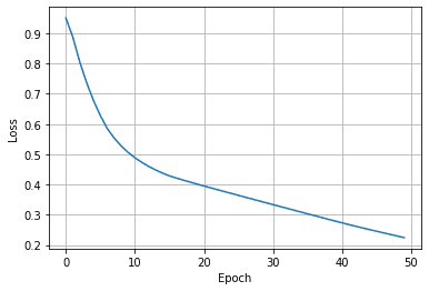
Figure 14: Loss plot (source: image by the authors).
→ Launch Jupyter Notebook on Google Colab → Launch Jupyter Notebook on Google Colab
Automatic Differentiation Part 2: Implementation Using Micrograd
# Inference
pred = mlp(xs[0])
ygt = ys[0]
print(f"Prediction => {pred.data: 0.2f}")
print(f"Ground Truth => {ygt: 0.2f}")
→ Launch Jupyter Notebook on Google Colab → Launch Jupyter Notebook on Google Colab
Automatic Differentiation Part 2: Implementation Using Micrograd
>>> Prediction => 0.14
>>> Ground Truth => 0.00
Summary
Our main objective with this blog post was to look under the hood of the autodiff process. With the help of Andrej’s
micrograd
repository, we now know how to shape a very minimal but working autodiff package.
We hope that the core concepts of autodiff, backpropagation, and basic neural network training are clear to you now.
Let us know how you liked this tutorial.


 829
829

 被折叠的 条评论
为什么被折叠?
被折叠的 条评论
为什么被折叠?
 到【灌水乐园】发言


