机器学习中的小波变换

这是一个学习总结。

原文链接：

A guide for using the Wavelet Transform in Machine Learning – ML Fundamentals

¢ 傅里叶变换只适合频谱是静态的情况。也就是说信号中的频率不是随着时间变化的；如果一个信号中含有一个 xHz 的频率，这个频率会均匀地出现在信号的任何地方。

¢ 生活中的信号多数是非静态的

¢ 所以使用小波变换会更好

从傅里叶变换到小波变换------------------------------------------------------------------------

¢ by multiplying a signal with a series of sine-waves with different frequencies we are able to determine which frequencies are present in a signal. If the dot-product between our signal and a sine wave of a certain frequency results in a large amplitude this means that there is a lot of overlap between the two signals, and our signal contains this specific frequency. This is of course because the dot product is a measure of how much two vectors / signals overlap .

¢ 傅里叶变换告诉我们信号中含有什么频率 ，但是没有告诉我们频率发生的时间

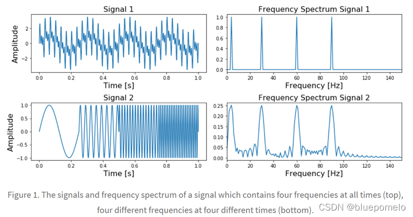
如上图，两个不同的信号，使用傅里叶变换，频谱图都类似，都是在4，30，60和90Hz出现峰值。傅里叶变换不能区分这两个信号。

Figure 2. A schematic overview of the time and frequency resolutions of the different transformations in comparison with the original time-series dataset. The size and orientations of the block gives an indication of the resolution size.

The size and orientation of the blocks indicate how small the features are that we can distinguish in the time and frequency domain.

The original time-series has a high resolution in the time-domain and zero resolution in the frequency domain. This means that we can distinguish very small features in the time-domain and no features in the frequency domain.

Opposite to that is the Fourier Transform, which has a high resolution in the frequency domain and zero resolution in the time-domain.

The Short Time Fourier Transform has medium sized resolution in both the frequency and time domain.

The Wavelet Transform has:

for small frequency values a high resolution in the frequency domain, low resolution in the time- domain, for large frequency values a low resolution in the frequency domain, high resolution in the time domain.

In other words, the Wavelet Transforms makes a trade-off; at scales in which time-dependent features are interesting it has a high resolution in the time-domain and at scales in which frequency-dependent features are interesting it has a high resolution in the frequency domain.

小波变换如何工作------------------------------------------------------------------------------

¢ 傅里叶变换利用不同频率的 sin 波去分析信号。一个信号是 sin 波的线性组合。

¢ 小波变换利用一些 wavelets （小波），每个 wavelet有 不同的规模。

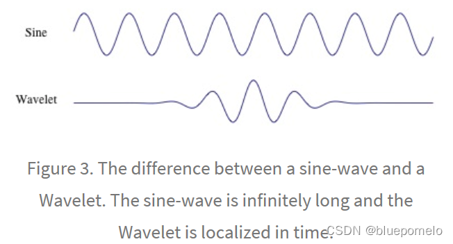
Sin wave在时间上不能定位，就是stretch from -infinity to infinity。小波则在时间上能定位（localized in time）

 

¢ 小波在时间上能定位，我们可以用时间上位置不同的小波与信号相乘。

¢ 从信号的头滑动小波到信号的尾。这个过程叫卷积。

 

¢ 傅里叶变换用频率，小波变换使用 scale 。频率更符合直觉，可以把 scale 转成频率。

¢ 高的 scale-factor 对应小的频率

¢ 可以说频率的倒数是 scale

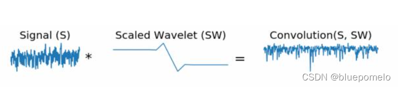
 so by scaling the wavelet in the time-domain we will analyze smaller frequencies (achieve a higher resolution) in the frequency domain. And vice versa, by using a smaller scale we have more detail in the time-domain.

小波家族-------------------------------------------------------------------------------

¢ 我们可以根据需要选择小波家族中的不同的小波

¢ PyWavelets 提供 14 中 mother wavelets

 Each type of wavelets has a different shape, smoothness and compactness and is useful for a different purpose. The wavelet families differ from each other since for each family a different trade-off has been made in how compact and smooth the wavelet looks like.

¢ A wavelet must have 1) finite energy and 2) zero mean.

¢ Finite energy means that it is localized in time and frequency; it is integrable and the inner product between the wavelet and the signal always exists.

¢ The admissibility condition implies a wavelet has zero mean in the time-domain, a zero at zero frequency in the time-domain. This is necessary to ensure that it is integrable and the inverse of the wavelet transform can also be calculated.

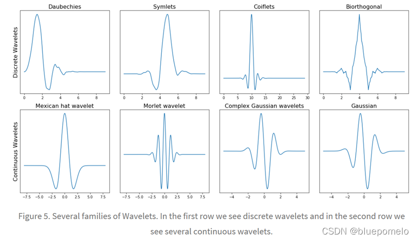
 ¢Within each wavelet family there can be a lot of different wavelet subcategories belonging to that family. You can distinguish the different subcategories of wavelets by the number of coefficients (the number of vanishing moments) and the level of decomposition.

 

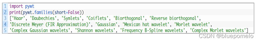
db1,db2,db3,db4,db5…db20,PyWavelets有20中db小波

db3 has three vanishing moments and db5 has 5 vanishing moment. The number of vanishing moments is related to the approximation order and smoothness of the wavelet. If a wavelet has p vanishing moments, it can approximate polynomials of degree p – 1.

When selecting a wavelet, we can also indicate what the level of decomposition has to be. By default, PyWavelets chooses the maximum level of decomposition possible for the input signal. The maximum level of decomposition (see pywt.dwt_max_level()) depends on the length of the input signal length and the wavelet (more on this later).

As we can see, as the number of vanishing moments increases, the polynomial degree of the wavelet increases and it becomes smoother. And as the level of decomposition increases, the number of samples this wavelet is expressed in increases.

连续小波v.s离散小波---------------------------------------------------------------------------

¢连续小波变换

 

 

¢ When we are talking about the Discrete Wavelet Transform, the main difference is that the DWT uses discrete values for the scale and translation factor. The scale factor increases in powers of two, so  a=1,2,4 and the translation factor increases integer values ( b=1,2,3 ).

¢ PS:  The DWT is only discrete in the scale and translation domain, not in the time-domain. To be able to work with digital and discrete signals we also need to discretize our wavelet transforms in the time-domain. These forms of the wavelet transform are called the Discrete-Time Wavelet Transform and the Discrete-Time Continuous Wavelet Transform.

离散小波变换（DWT）作为一个过滤机---------------------------------------------------

¢ DWT 通常以一个级联的高通过滤器和低通过滤器实现

¢ 过滤机把信号分成不同频率的通道

¢ 在信号上使用 DWT ，从小的 scale 开始。小的 scale 对应高的频率。这意味着首先分析高频行为。第二阶段， scale 增加 2 的倍数（频率降低 2 的倍数）。我们分析的是大概最大频率的一半。第三阶段， scale 是 4 ，我们分析的大概是最大频率的 1/4 。就这样一直下去，直到我们到达最大的分解层级 。

¢ 什么是最大分解层级？在每个阶段，信号的样本点两倍的速度减少。在低的频率值，你需要少一点的样本点满足 Nyquist rate 。由于这个样本下降，在某个阶段信号中的样本量减少到比波过滤器的长度要短，此时到达最大分解层级。

¢ 例子：有一个信号最高频率是 1000Hz 。第一阶段，把信号分成低频部分和高频部分，即 0-500Hz 以及 500-1000Hz 。第二阶段，我们把低频的部分在分成两部分： 0-250Hz 和 250-500Hz 。第三阶段，把低频部分 0-250Hz 分成 0-125Hz 和 125-250Hz 两部分。这个过程继续直到样本点降到没有样本可用。

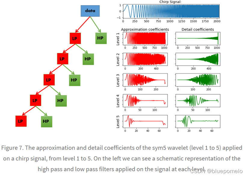
A chirp signal is a signal with a dynamic frequency spectrum; the frequency spectrum increases with time. The start of the signal contains low frequency values and the end of the signal contains the high frequencies. This makes it easy for us to visualize which part of the frequency spectrum is filtered out by simply looking at the time-axis. 

¢In PyWavelets the DWT is applied with pywt.dwt()

¢The DWT return two sets of coefficients; the approximation coefficients and detail coefficients.

¢The approximation coefficients represent the output of the low pass filter (averaging filter) of the DWT.

¢The detail coefficients represent the output of the high pass filter (difference filter) of the DWT.

¢By applying the DWT again on the approximation coefficients of the previous DWT, we get the wavelet transform of the next level.

¢At each next level, the original signal is also sampled down by a factor of 2.

¢PS: We can also use pywt.wavedec() to immediately calculate the coefficients of a higher level. This functions takes as input the original signal and the level  and returns the one set of approximation coefficients (of the n-th level) and n sets of detail coefficients (1 to n-th level).

¢PS2: This idea of analyzing the signal on different scales is also known as multiresolution / multiscale analysis, and decomposing your signal in such a way is also known as multiresolution decomposition, or sub-band coding.

应用-------------------------------------------------------------------

¢3.1 使用连续小波变换可视化状态空间

¢3.2使用连续小波变换与CNN对信号分类

¢3.3使用离散小波变换分解信号

¢3.4利用离散小波变换去除高频噪音

¢3.5使用离散傅里叶变换做信号分类

   3.5.3使用多种特征和scikit-learn分类器去分类两种ECG库

总结

A lot will depend on the choices you make; which wavelet transform will you use, CWT or DWT? which wavelet family will you use? Up to which level of decomposition will you go? What is the right range of scales to use?