pytorch神经网络入门(八)

目录

一、概述

二、代码

​三、总结

四、附图

---

一、概述

使用minist数据集进行分类训练并且展示预测结果

二、代码

import  torch
from    torch import nn
from    torch.nn import functional as F
from    torch import optim
import  torchvision
from    matplotlib import pyplot as plt
from    utils import plot_image, plot_curve, one_hot

batch_size = 512

# step1. load dataset
train_loader = torch.utils.data.DataLoader(
    torchvision.datasets.MNIST('mnist_data', train=True, download=True,
                               transform=torchvision.transforms.Compose([
                                   torchvision.transforms.ToTensor(),
                                   torchvision.transforms.Normalize(
                                   (0.1307,), (0.3081,))
                               ])),
    batch_size=batch_size, shuffle=True)å

test_loader = torch.utils.data.DataLoader(
    torchvision.datasets.MNIST('mnist_data/', train=False, download=True,
                               transform=torchvision.transforms.Compose([
                                   torchvision.transforms.ToTensor(),
                                   torchvision.transforms.Normalize(
                                       (0.1307,), (0.3081,))
                               ])),
    batch_size=batch_size, shuffle=False)



class Net(nn.Module):

    def __init__(self):
        super(Net, self).__init__()

        # xw+b
        self.fc1 = nn.Linear(28*28, 256)
        self.fc2 = nn.Linear(256, 64)
        self.fc3 = nn.Linear(64, 10)

    def forward(self, x):
        # x: [b, 1, 28, 28]
        # h1 = relu(xw1+b1)
        x = F.relu(self.fc1(x))
        # h2 = relu(h1w2+b2)
        x = F.relu(self.fc2(x))
        # h3 = h2w3+b3
        x = self.fc3(x)

        return x

net = Net()

def training():

    # [w1, b1, w2, b2, w3, b3]
    optimizer = optim.SGD(net.parameters(), lr=0.01, momentum=0.9)

    train_loss = []
    for epoch in range(3):
        for batch_idx, (x, y) in enumerate(train_loader):
            # x: [b, 1, 28, 28], y: [512]
            # [b, 1, 28, 28] => [b, 784]
            x = x.view(x.size(0), 28 * 28)
            # => [b, 10]
            out = net(x)
            # [b, 10]
            y_onehot = one_hot(y)
            # loss = mse(out, y_onehot)
            loss = F.mse_loss(out, y_onehot)

            optimizer.zero_grad()
            loss.backward()
            # w' = w - lr*grad
            optimizer.step()
            train_loss.append(loss.item())
            if batch_idx % 10 == 0:
                print(epoch, batch_idx, loss.item())

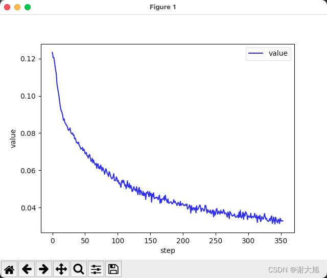
    plot_curve(train_loss)

def testing():
    # we get optimal [w1, b1, w2, b2, w3, b3]
    total_correct = 0
    for x, y in test_loader:
        x = x.view(x.size(0), 28 * 28)
        out = net(x)
        # out: [b, 10] => pred: [b]
        pred = out.argmax(dim=1)
        correct = pred.eq(y).sum().float().item()
        total_correct += correct
    total_num = len(test_loader.dataset)
    acc = total_correct / total_num
    print('test acc:', acc)


if __name__=="__main__":

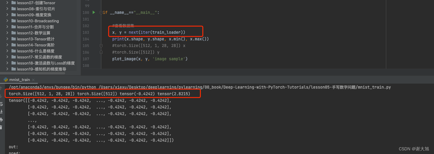
    #查看数据集
    x, y = next(iter(train_loader))
    print(x.shape, y.shape, x.min(), x.max())
    #torch.Size([512, 1, 28, 28]) x
    #torch.Size([512]) y
    plot_image(x, y, 'image sample')

    #网络为经过训练
    x, y = next(iter(test_loader))
    #[512 10]
    # x.view(x.size(0), 28 * 28)=====>[512,784]
    #[512,784]==>[784,256]
    #[784,256]==>[265,64]
    #[265,64]==>[64,10]
    out = net(x.view(x.size(0), 28 * 28))
    #返回最大值所在的序号，认为该需要（标注）就是当前图片对应的值 【512，1】
    pred = out.argmax(dim=1)
    plot_image(x, pred, 'test')
    #训练网络和测试网络
    training()
    testing()
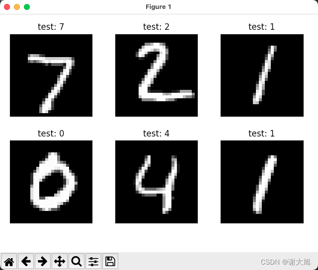
    #再次显示图片
    x, y = next(iter(test_loader))
    out = net(x.view(x.size(0), 28 * 28))
    pred = out.argmax(dim=1)
    plot_image(x, pred, 'test')

import  torch
from    matplotlib import pyplot as plt

def plot_curve(data):
    fig = plt.figure()
    plt.plot(range(len(data)), data, color='blue')
    plt.legend(['value'], loc='upper right')
    plt.xlabel('step')
    plt.ylabel('value')
    plt.show()


def plot_image(img, label, name):

    fig = plt.figure()
    for i in range(6):
        plt.subplot(2, 3, i + 1)
        plt.tight_layout()
        plt.imshow(img[i][0]*0.3081+0.1307, cmap='gray', interpolation='none')
        plt.title("{}: {}".format(name, label[i].item()))
        plt.xticks([])
        plt.yticks([])
    plt.show()


def one_hot(label, depth=10):
    out = torch.zeros(label.size(0), depth)
    idx = torch.LongTensor(label).view(-1, 1)
    out.scatter_(dim=1, index=idx, value=1)
    return out

注意：

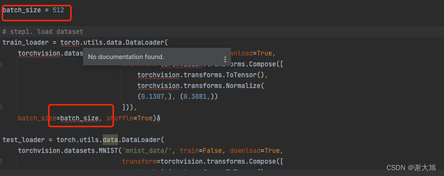
这里决定了在trainloader里边取一次数据的数据量是 512

三、总结

学习过程要多关注神经网络的输入和输出所代表的物理含义

熟悉python语言以及三方包的接口

四、附图