复杂网络特征与networkx实现------（二）

---

图的类型

• Graph类是无向图的基类，无向图能有自己的属性或参数，不包含重边，允许有回路，节点可以是任何hash的python对象，节点和边可以保存key/value属性对。该类的构造函数为Graph(data=None，**attr)，其中data可以是边列表，或任意一个Networkx的图对象，默认为none；attr是关键字参数，例如key=value对形式的属性。

import networkx as nx      #导入NetworkX包，为了少打几个字母，将其重命名为nx
G = nx.Graph()              #建立一个空的无向图G

• MultiGraph是可以有重边的无向图，其它和Graph类似。其构造函数MultiGraph（data=None, *attr）。

• DiGraph是有向图的基类，有向图可以有数自己的属性或参数，不包含重边，允许有回路；节点可以是任何hash的python对象，边和节点可含key/value属性对。该类的构造函数DiGraph(data=None,**attr)，其中data可以是边列表，或任意一个Networkx的图对象，默认为none；attr是关键字参数，例如key=value对形式的属性。

• MultiDiGraph是可以有重边的有向图，其它和DiGraph类似。其构造函数MultiDiGraph（data=None, *attr）。

---

基本概念

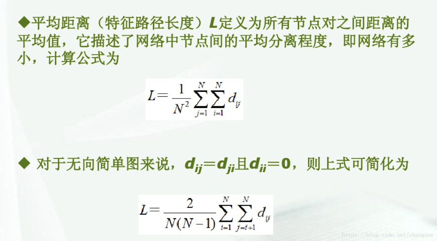
• 距离
  最短距离：两节点$v_i$和节点$v_j$经历边数最少的一条简单路径
  直径：任意两个节点距离的最大值$D= max_{i,j}{d_(ij)}$
  

• 度
  节点度：无向图中，与节点v 相连的节点数量d(v)或 $k_i$
  有向图中 分 出度和入度，入度 其他节点指向节点v的个数 $d _ in (v)$
  出度，节点v指向其他节点的个数

  网络平均度$D^-=avg_{i,j}{d_(ij)}$

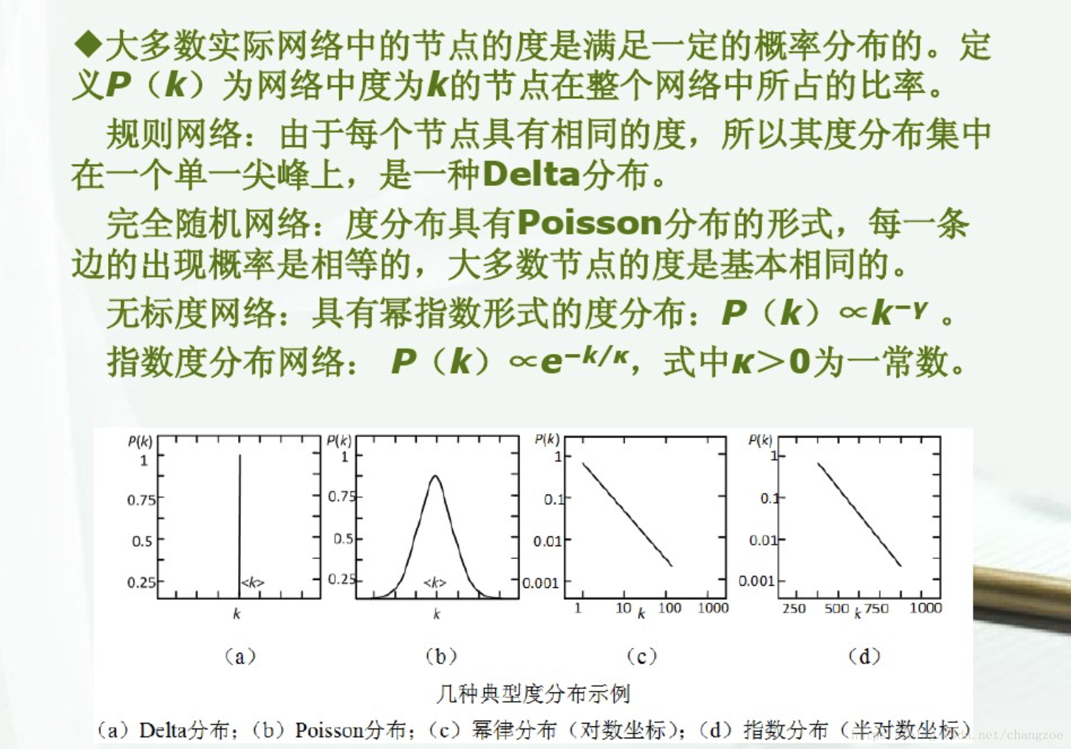
  度分布
  

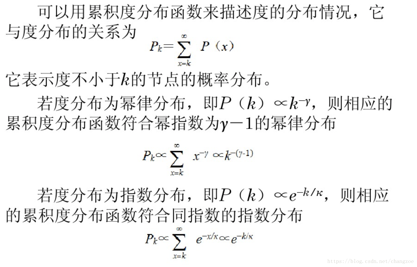
  累计度分布

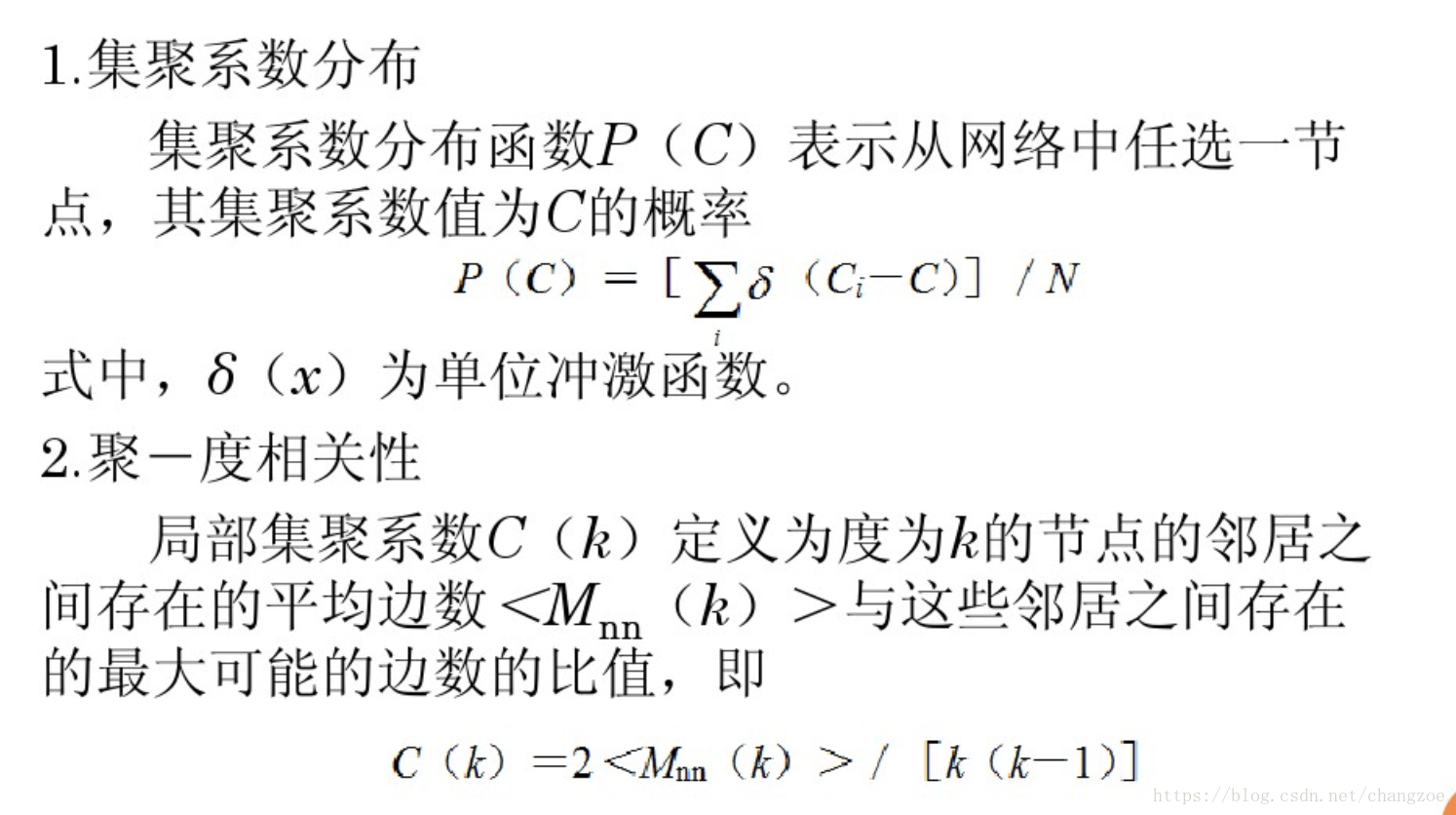
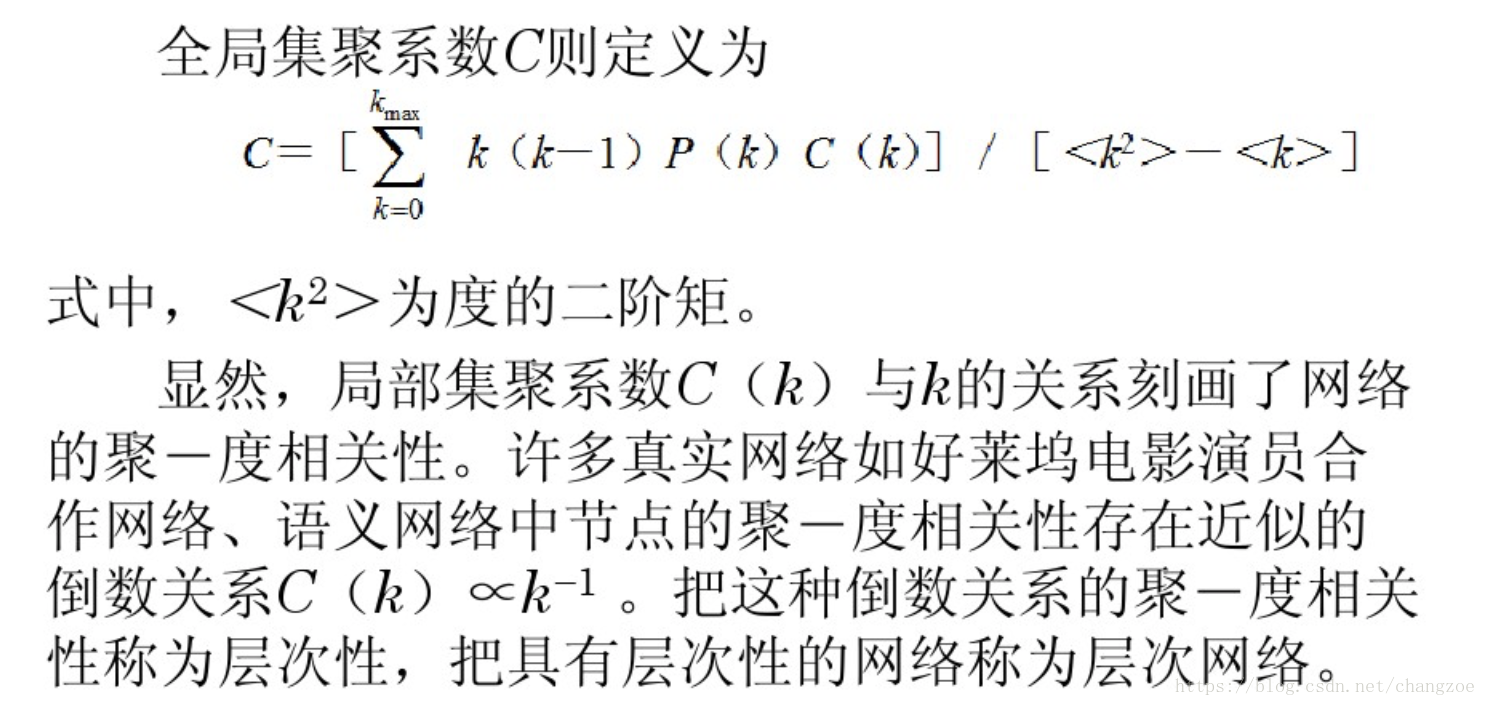
• 聚集系数
  网络G =（V，E）
  d($v_i$)表示$v_i$的度值
  与节点$v_i$相连的顶点有d($v_i$), 这些节点实际相恋的次数为$M_i$，
  最多可能的边数为 $d(v_i)(d(v_i)-1)/2$
  节点$v_i$的聚集系数为
  $$c_i= \frac{2M_i}{d(v_i)(d(v_i)-1)}$$

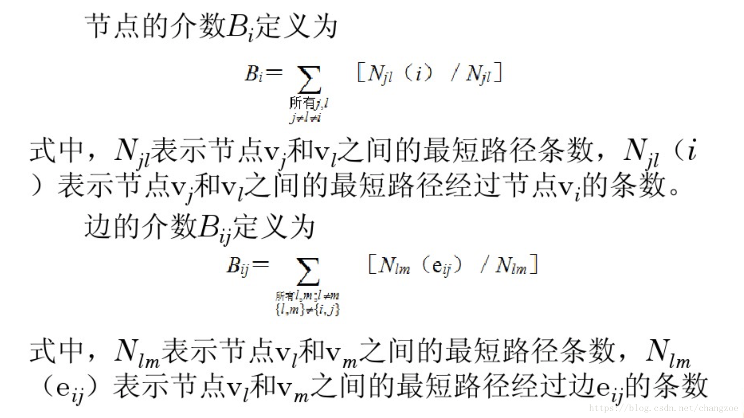
• 介数

• 核数

• 度中心性
  节点$v_i$的度中心性：
  $$d(v_i)/(N-1)$$

网络G 含N个节点的 度中心：

$$C_D=\sum_{I=1}^N [C_D(V_max)-C_D(V_i)] /H$$

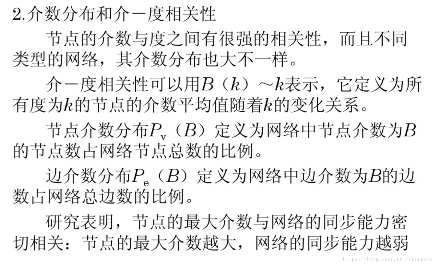
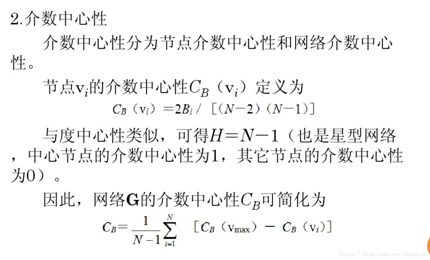
• 介数中心性
  

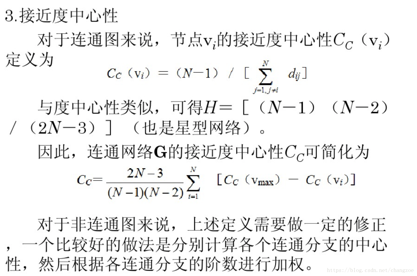
• 接近度指标
  

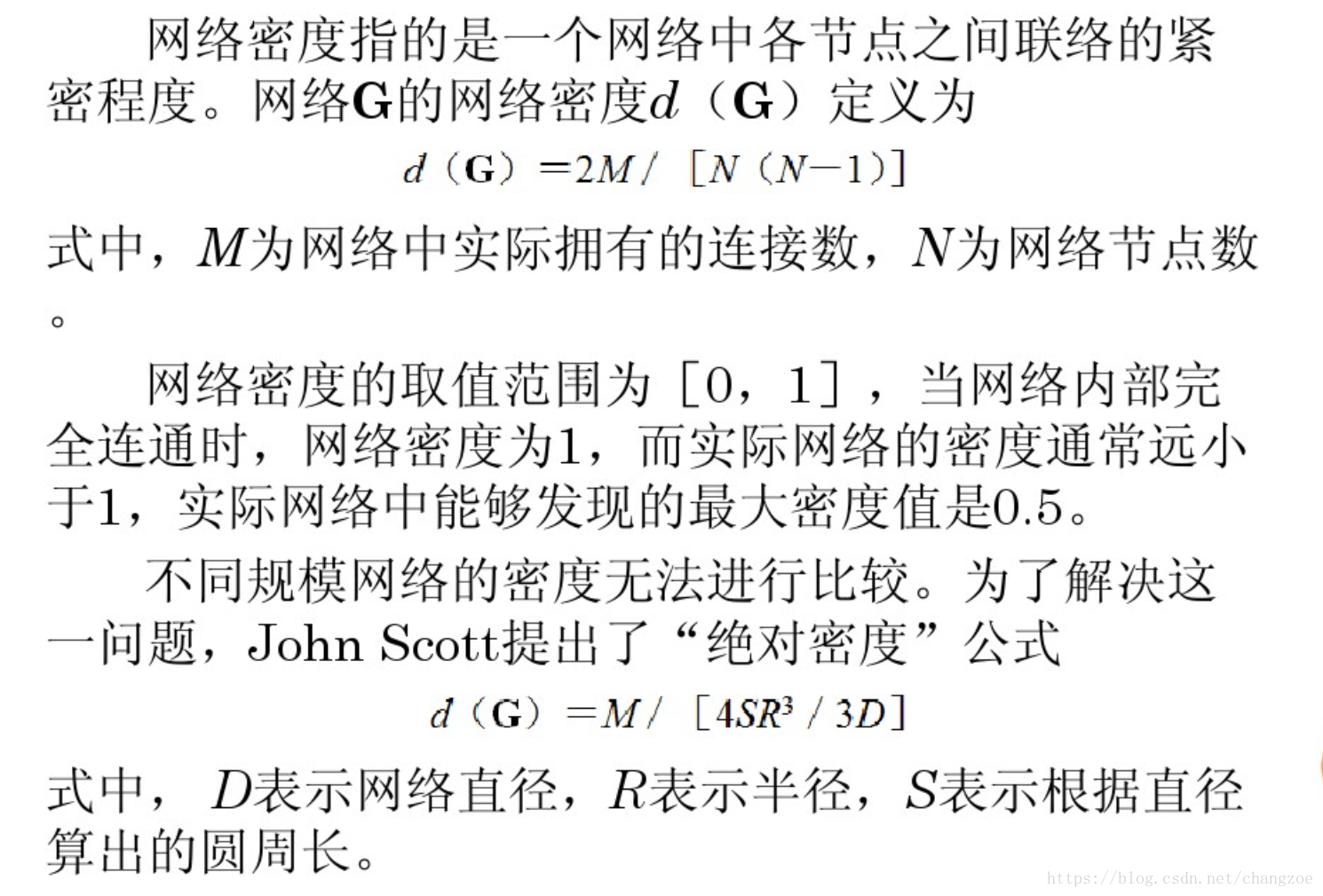
• 密度
  

---

---

networkx实现

import networkx as nx #使用库的声明  
G=nx.Graph()  #初始化  
G=nx.Graph(name='my graph')  
e=[(1,2),(1,3),(2,3),(3,4),(4,5)]  
G=nx.Graph(e)  #为图G添加边  

#节点数
len(G)
##边数
G.number_of_edges()
###节点表
G.nodes()
##边表
G.edges()
Out[27]: EdgeView([(1, 2), (1, 3), (2, 3), (3, 4), (4, 5)])

画图

nx.draw(G)

图的密度
计算图的密度，其值为边数m除以图中可能边数（即n(n-1)/2）

diameter(G)
Out[29]: 0.5

最短路径

shortest_path(G, source=None, target=None, weight=None)

Parameters :    

G : NetworkX graph

source : node, optional

Starting node for path. If not specified, compute shortest paths using all nodes as source nodes.

target : node, optional

Ending node for path. If not specified, compute shortest paths using all nodes as target nodes.

weight : None or string, optional (default = None)

If None, every edge has weight/distance/cost 1. If a string, use this edge attribute as the edge weight. Any edge attribute not present defaults to 1.

Returns :   
path: list or dictionary

print(nx.shortest_path(G,source=5,target=1))
[5, 4, 3, 1]

p=nx.shortest_path(G,source=1) 
p[2]
Out[73]: [1, 2]

#所有节点间的最短*路径*,列表存储
nx.all_pairs_shortest_path(G)
Out[33]: <generator object all_pairs_shortest_path at 0x151ef99c50>
>>> G=nx.path_graph(5)
>>> path=nx.all_pairs_shortest_path(G)
>>> print(path[0][4])
[0, 1, 2, 3, 4]
#网络节点间的平均最短路长度
nx.average_shortest_path_length(G)
Out[34]: 1.7

度分布

Degree_distribution = nx.degree_histogram(G)
A list of frequencies of degrees. The degree values are the index in the list.
Out[86]: [0, 1, 3, 1]

度中心性
节点$v_i$的度中心性：

$$d(v_i)/(N-1)$$

nx.degree_centrality(G)  
{1: 0.5, 2: 0.5, 3: 0.75, 4: 0.5, 5: 0.25}  

插边

#插入边，点会自动生成
G.add_edge(4, 6)
G.add_edge(6,7 )

聚集系数
节点$v_i$的聚集系数为

$$c_i= \frac{2M_i}{d(v_i)(d(v_i)-1)}$$

nx.clustering(G)
{1: 1.0, 2: 1.0, 3: 0.3333333333333333, 4: 0, 5: 0, 6: 0, 7: 0}

closing
通过距离来表示节点在图中的重要性，一般是指节点到其他节点的平均路径的倒数，这里还乘以了n-1。该值越大表示节点到其他节点的距离越近，即中心性越高。

nx.closeness_centrality(G)
Out[98]: 
{1: 0.42857142857142855,
 2: 0.42857142857142855,
 3: 0.6,
 4: 0.6666666666666666,
 5: 0.42857142857142855,
 6: 0.5,
 7: 0.35294117647058826}

nx.betweenness_centrality(G)
节点介数中心系数。在无向图中，该值表示为节点作占最短路径的个数除以((n-1)(n-2)/2)；在有向图中，该值表达为节点作占最短路径个数除以((n-1)(n-2))。

nx.betweenness_centrality(G)

{1: 0.0,
 2: 0.0,
 3: 0.5333333333333333,
 4: 0.7333333333333333,
 5: 0.0,
 6: 0.3333333333333333,
 7: 0.0}

传递性

nx.transitivity(G)

0.3333333333333333

图或网络的传递性。即图或网络中，认识同一个节点的两个节点也可能认识双方，计算公式为3*图中三角形的个数/三元组个数（该三元组个数是有公共顶点的边对数，这样就好数了）。

---

绘图

"""
Created on Thu Jul 19 20:49:23 2018

@author: cc
"""

import networkx as nx                   #导入networkx包
import matplotlib.pyplot as plt     #导入绘图包matplotlib（需要安装，方法见第一篇笔记）
G =nx.random_graphs.barabasi_albert_graph(100,1)   #生成一个BA无标度网络G
nx.draw(G)                          #绘制网络G
plt.savefig("ba.png")           #输出方式1: 将图像存为一个png格式的图片文件
plt.show()                            #输出方式2: 在窗口中显示这幅图像             

运用样式
上边的代码虽然简单，但生成的图形略显单调。NetworkX提供了一系列样式参数，可以用来修饰和美化图形，达到我们想要的效果。常用的参数包括：
- node_size: 指定节点的尺寸大小(默认是300，单位未知，就是上图中那么大的点)
- node_color: 指定节点的颜色 (默认是红色，可以用字符串简单标识颜色，例如’r’为红色，’b’为绿色等，具体可查看手册)
- node_shape: 节点的形状（默认是圆形，用字符串’o’标识，具体可查看手册）
- alpha: 透明度 (默认是1.0，不透明，0为完全透明)
- width: 边的宽度 (默认为1.0)
- edge_color: 边的颜色(默认为黑色)
- style: 边的样式(默认为实现，可选： solid|dashed|dotted,dashdot)
- with_labels: 节点是否带标签（默认为True）
- font_size: 节点标签字体大小 (默认为12)
- font_color: 节点标签字体颜色（默认为黑色）
灵活运用上述参数，可以绘制不同样式的网络图形，例如：nx.draw(G,node_size = 30,with_labels = False) 是绘制节点尺寸为30、不带标签的网络图。

三、运用布局
NetworkX在绘制网络图形方面提供了布局的功能，可以指定节点排列的形式。这些布局包括：
circular_layout：节点在一个圆环上均匀分布
random_layout：节点随机分布
shell_layout：节点在同心圆上分布
spring_layout： 用Fruchterman-Reingold算法排列节点（这个算法我不了解，样子类似多中心放射状）
spectral_layout：根据图的拉普拉斯特征向量排列节点？我也不是太明白
布局用pos参数指定，例如：nx.draw(G,pos = nx.circular_layout(G))。在上一篇笔记中，四个不同的模型分别是用四种布局绘制的，可以到那里去看一下效果，此处就不再重复写代码了。
另外，也可以单独为图中的每个节点指定一个位置（x、y坐标），感兴趣的朋友可以看一下NetworkX文档中的一个例子：
http://networkx.lanl.gov/examples/drawing/knuth_miles.html。

draw(G, pos=None, ax=None, hold=None, **kwds)

Parameters :    
G : graph

A networkx graph

pos : dictionary, optional

A dictionary with nodes as keys and positions as values. If not specified a spring layout positioning will be computed. See networkx.layout for functions that compute node positions.

ax : Matplotlib Axes object, optional

Draw the graph in specified Matplotlib axes.

hold : bool, optional

Set the Matplotlib hold state. If True subsequent draw commands will be added to the current axes.

**kwds : optional keywords

See networkx.draw_networkx() for a description of optional keywords.

四、添加文本
用 plt.title()方法可以为图形添加一个标题，该方法接受一个字符串作为参数，fontsize参数用来指定标题的大小。例如：plt.title(“BA Networks”, fontsize = 20)。如果要在任意位置添加文本，则可以采用plt.text()方法。事实上这些功能（包括前边的图形保存等功能）并不是由NetworkX提供的，从包的名字上可以看出，这些绘图函数都是由matplotlib这个包提供的。NetworkX只是把与复杂网络绘图相关的功能重新包装了一下，让用户调用更方便而已。
需要补充的一点是，matplotlib并不直接支持中文文本，如果想输出中文，走正规方法还是挺麻烦的（见http://blog.csdn.net/KongDong/archive/2009/07/10/4338826.aspx）。不过有聪明的网友提出了一种偷梁换柱的解决方案：换字体。只要把一个中文字体文件（ttf文件）更名为Vera.ttf，拷贝到matplotlib的字体目录中覆盖原有文件，就可以输出中文了，具体细节见http://hi.baidu.com/ucherish/blog/item/63155e52b68c90070df3e3ff.html 。

---

参考文献

https://networkx.github.io/documentation/networkx-1.9/reference/generated/networkx.classes.function.degree_histogram.html?highlight=degree_histogram

文档

https://www.cnblogs.com/gispathfinder/p/5790949.html