


信用卡交易中的异常检测如何工作?
这是星期天早上,它很安静,你醒来时脸上露出灿烂的笑容。今天将是美好的一天!除此之外,您的手机响起,而非“国际化”。你慢慢地捡起它,听到一些非常奇怪的东西 - “Bonjour,je suis Michele。哎呀,对不起。我是米歇尔,你的私人银行代理人。“ 瑞士有人在这个时候给你打电话可能会如此迫切?“你是否以100美元的暗黑破坏神3的价格授权了3,358.65美元的交易?”马上,你开始想办法解释为什么你这样做会给你所爱的人。“不,我没有!?” 米歇尔的答案很快而且非常重要 - “谢谢你,我们就是这样”。哇,那很接近!但米歇尔怎么知道这笔交易是可疑的呢?毕竟,你上周从同一个银行账户订购了10部新智能手机 - 米歇尔当时没有打电话。
想要获取本文完整的代码和数据,请加入TensorFlow QQ群:469331966

来源:Tutsplus
根据尼尔森报告,2015年全球欺诈损失达到218亿美元。如果你是骗子,你可能会觉得很幸运。同年,美国每100美元大约每12美分被盗一次。我们的朋友米歇尔可能在这里要解决一个严重的问题。
在本系列的这一部分中,我们将以无人监督(或半监督)的方式训练自动编码器神经网络(在Keras中实施),用于信用卡交易数据中的异常检测。训练后的模型将在预先标记和匿名的数据集上进行评估。
建立
我们将使用TensorFlow 1.2和Keras 2.0.4。让我们开始:
<span style="color:rgba(0, 0, 0, 0.84)"><code><strong>import</strong> <strong>pandas</strong> <strong>as</strong> <strong>pd</strong>
<strong>import</strong> <strong>numpy</strong> <strong>as</strong> <strong>np</strong>
<strong>import</strong> <strong>pickle</strong>
<strong>import</strong> <strong>matplotlib.pyplot</strong> <strong>as</strong> <strong>plt</strong>
<strong>from</strong> <strong>scipy</strong> <strong>import</strong> stats
<strong>import</strong> <strong>tensorflow</strong> <strong>as</strong> <strong>tf</strong>
<strong>import</strong> <strong>seaborn</strong> <strong>as</strong> <strong>sns</strong>
<strong>from</strong> <strong>pylab</strong> <strong>import</strong> rcParams
<strong>from</strong> <strong>sklearn.model_selection</strong> <strong>import</strong> train_test_split
<strong>from</strong> <strong>keras.models</strong> <strong>import</strong> Model, load_model
<strong>from</strong> <strong>keras.layers</strong> <strong>import</strong> Input, Dense
<strong>from</strong> <strong>keras.callbacks</strong> <strong>import</strong> ModelCheckpoint, TensorBoard
<strong>from</strong> <strong>keras</strong> <strong>import</strong> regularizers</code></span>
<span style="color:rgba(0, 0, 0, 0.84)"><code>%matplotlib inline</code></span><span style="color:rgba(0, 0, 0, 0.84)"><code>sns.set(style='whitegrid', palette='muted', font_scale=1.5)</code></span><span style="color:rgba(0, 0, 0, 0.84)"><code>rcParams['figure.figsize'] = 14, 8</code></span><span style="color:rgba(0, 0, 0, 0.84)"><code>RANDOM_SEED = 42
LABELS = ["Normal", "Fraud"]</code></span>加载数据
我们将要使用的数据集可以从Kaggle下载。它包含有关在两天内发生的信用卡交易的数据,在284,807笔交易中有492个欺诈。
数据集中的所有变量都是数字的。由于隐私原因,数据已使用PCA转换进行转换。未更改的两个功能是时间和金额。时间包含每个事务与数据集中第一个事务之间经过的秒数。
<span style="color:rgba(0, 0, 0, 0.84)"><code>df = pd.read_csv("data/creditcard.csv")</code></span>勘探
<span style="color:rgba(0, 0, 0, 0.84)"><code>df.shape</code></span>>(284807, 31)
31列,其中2列是时间和金额。其余的是PCA转换输出。我们来检查缺失的值:
<span style="color:rgba(0, 0, 0, 0.84)"><code>df.isnull().values.any()</code></span>> False
<span style="color:rgba(0, 0, 0, 0.84)"><code>count_classes = pd.value_counts(df['Class'], sort = True)
count_classes.plot(kind = 'bar', rot=0)
plt.title("Transaction class distribution")
plt.xticks(range(2), LABELS)
plt.xlabel("Class")
plt.ylabel("Frequency");</code></span>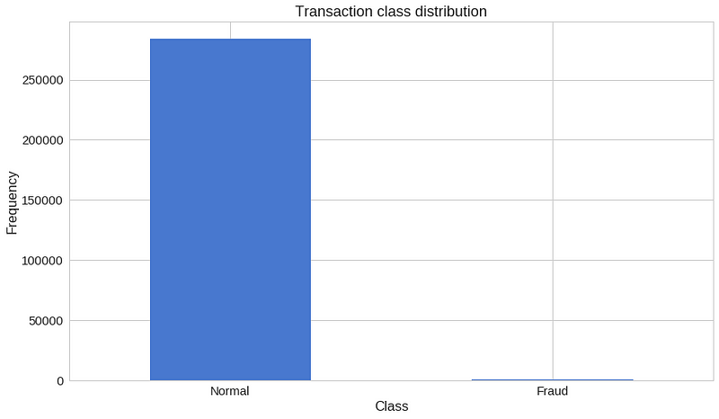
我们手上有一个高度不平衡的数据集。正常交易大大超过了欺诈性交易。我们来看看两种类型的交易:
<span style="color:rgba(0, 0, 0, 0.84)"><code>frauds = df[df.Class == 1]
normal = df[df.Class == 0]</code></span>
<span style="color:rgba(0, 0, 0, 0.84)"><code>frauds.shape</code></span>> (492, 31)
<span style="color:rgba(0, 0, 0, 0.84)"><code>normal.shape</code></span>> (284315, 31)
不同交易类别的使用金额有何不同?
<span style="color:rgba(0, 0, 0, 0.84)"><code>frauds.Amount.describe()</code></span>>
<span style="color:rgba(0, 0, 0, 0.84)"><code>count     492.000000
mean      122.211321
std       256.683288
min         0.000000
25%         1.000000
50%         9.250000
75%       105.890000
max      2125.870000
Name: Amount, dtype: float64</code></span>
>
<span style="color:rgba(0, 0, 0, 0.84)"><code>normal.Amount.describe()</code></span>>
<span style="color:rgba(0, 0, 0, 0.84)"><code>count    284315.000000
mean         88.291022
std         250.105092
min           0.000000
25%           5.650000
50%          22.000000
75%          77.050000
max       25691.160000
Name: Amount, dtype: float64</code></span>
让我们有一个更多的图形表示:
<span style="color:rgba(0, 0, 0, 0.84)"><code>f, (ax1, ax2) = plt.subplots(2, 1, sharex=True)
f.suptitle('Amount per transaction by class')

bins = 50

ax1.hist(frauds.Amount, bins = bins)
ax1.set_title('Fraud')

ax2.hist(normal.Amount, bins = bins)
ax2.set_title('Normal')

plt.xlabel('Amount ($)')
plt.ylabel('Number of Transactions')
plt.xlim((0, 20000))
plt.yscale('log')
plt.show();</code></span>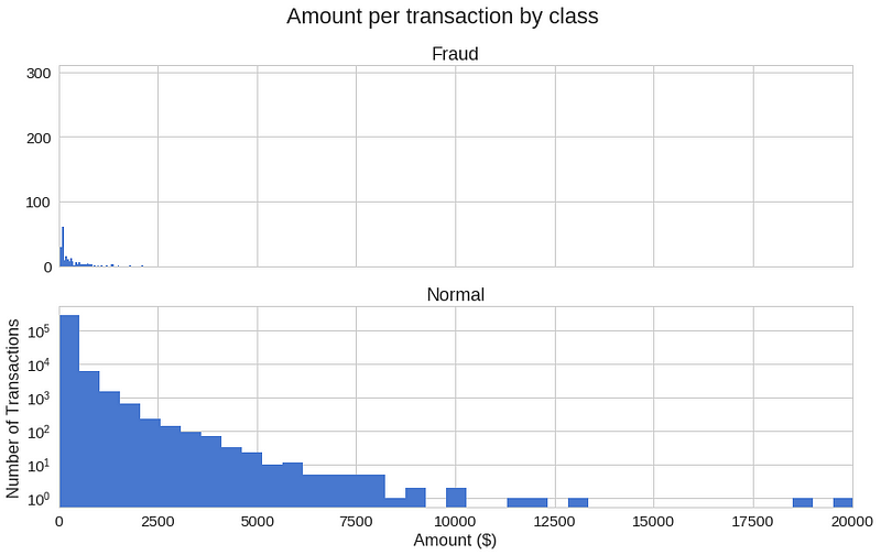
欺诈交易是否会在特定时间内更频繁地发生?
<span style="color:rgba(0, 0, 0, 0.84)"><code>f, (ax1, ax2) = plt.subplots(2, 1, sharex=True)
f.suptitle('Time of transaction vs Amount by class')

ax1.scatter(frauds.Time, frauds.Amount)
ax1.set_title('Fraud')

ax2.scatter(normal.Time, normal.Amount)
ax2.set_title('Normal')

plt.xlabel('Time (in Seconds)')
plt.ylabel('Amount')
plt.show()</code></span>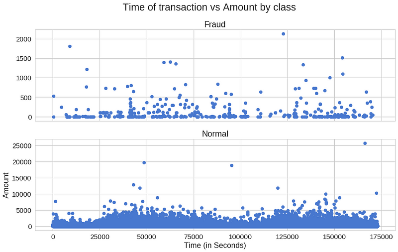
似乎交易时间真的很重要。
自动编码
Autoencoders起初看起来很奇怪。这些模型的工作是在给定相同输入的情况下预测输入。百思不得其解?对我来说绝对是第一次听到它。
更具体地说,让我们来看看自动编码器神经网络。此Autoencoder尝试学习近似以下身份函数:
![]()
虽然尝试做到这一点听起来可能听起来微不足道,但重要的是要注意我们想要学习数据的压缩表示,从而找到结构。这可以通过限制模型中隐藏单元的数量来完成。这些类型的自动编码的被称为undercomplete。
以下是Autoencoder可能学习的内容的直观表示:

重建错误
我们优化Autoencoder模型的参数,以便最大限度地减少特殊类型的错误 - 重建错误。在实践中,经常使用传统的平方误差:
![]()
如果您想了解有关Autoencoders的更多信息,我强烈推荐Hugo Larochelle的以下视频:
准备数据
首先,让我们删除Time列(不打算使用它)并在Amount上使用scikit的StandardScaler。缩放器删除均值并将值缩放为单位差异:
<span style="color:rgba(0, 0, 0, 0.84)"><code><strong>from</strong> <strong>sklearn.preprocessing</strong> <strong>import</strong> StandardScaler</code></span><span style="color:rgba(0, 0, 0, 0.84)"><code>data = df.drop(['Time'], axis=1)</code></span><span style="color:rgba(0, 0, 0, 0.84)"><code>data['Amount'] = StandardScaler().fit_transform(data['Amount'].values.reshape(-1, 1))</code></span>训练我们的Autoencoder会与我们习惯的有点不同。假设您有一个包含大量非欺诈性交易的数据集。您想要检测新事务的任何异常。我们将通过仅在正常交易上训练我们的模型来创建这种情况。在测试集上保留正确的类将为我们提供一种评估模型性能的方法。我们将保留20%的数据用于测试:
<span style="color:rgba(0, 0, 0, 0.84)"><code>X_train, X_test = train_test_split(data, test_size=0.2, random_state=RANDOM_SEED)
X_train = X_train[X_train.Class == 0]
X_train = X_train.drop(['Class'], axis=1)</code></span>
<span style="color:rgba(0, 0, 0, 0.84)"><code>y_test = X_test['Class']
X_test = X_test.drop(['Class'], axis=1)</code></span><span style="color:rgba(0, 0, 0, 0.84)"><code>X_train = X_train.values
X_test = X_test.values</code></span><span style="color:rgba(0, 0, 0, 0.84)"><code>X_train.shape</code></span>> (227451, 29)
建立模型
我们的Autoencoder使用4个完全连接的层,分别有14,7,7和29个神经元。前两层用于我们的编码器,最后两层用于解码器。此外,在训练期间将使用L1正则化:
<span style="color:rgba(0, 0, 0, 0.84)"><code>input_dim = X_train.shape[1]
encoding_dim = 14

</code></span>
<span style="color:rgba(0, 0, 0, 0.84)"><code>input_layer = Input(shape=(input_dim, ))</code></span><span style="color:rgba(0, 0, 0, 0.84)"><code>encoder = Dense(encoding_dim, activation="tanh",
activity_regularizer=regularizers.l1(10e-5))(input_layer)
encoder = Dense(int(encoding_dim / 2), activation="relu")(encoder)</code></span><span style="color:rgba(0, 0, 0, 0.84)"><code>decoder = Dense(int(encoding_dim / 2), activation='tanh')(encoder)
decoder = Dense(input_dim, activation='relu')(decoder)</code></span><span style="color:rgba(0, 0, 0, 0.84)"><code>autoencoder = Model(inputs=input_layer, outputs=decoder)</code></span>让我们训练我们的模型100个纪元,批量大小为32个样本,并将最佳表现模型保存到文件中。Keras提供的ModelCheckpoint对于此类任务非常方便。此外,培训进度将以TensorBoard理解的格式导出。
<span style="color:rgba(0, 0, 0, 0.84)"><code>nb_epoch = 100
batch_size = 32</code></span>
<span style="color:rgba(0, 0, 0, 0.84)"><code>autoencoder.compile(optimizer='adam',
loss='mean_squared_error',
metrics=['accuracy'])</code></span><span style="color:rgba(0, 0, 0, 0.84)"><code>checkpointer = ModelCheckpoint(filepath="model.h5",
verbose=0,
save_best_only=True)
tensorboard = TensorBoard(log_dir='./logs',
histogram_freq=0,
write_graph=True,
write_images=True)</code></span><span style="color:rgba(0, 0, 0, 0.84)"><code>history = autoencoder.fit(X_train, X_train,
epochs=nb_epoch,
batch_size=batch_size,
shuffle=True,
validation_data=(X_test, X_test),
verbose=1,
callbacks=[checkpointer, tensorboard]).history</code></span>并加载保存的模型(只是为了检查它是否有效):
<span style="color:rgba(0, 0, 0, 0.84)"><code>autoencoder = load_model('model.h5')</code></span>评估
<span style="color:rgba(0, 0, 0, 0.84)"><code>plt.plot(history['loss'])
plt.plot(history['val_loss'])
plt.title('model loss')
plt.ylabel('loss')
plt.xlabel('epoch')
plt.legend(['train', 'test'], loc='upper right');</code></span>
我们的训练和测试数据的重建错误似乎很好地收敛。它够低吗?让我们仔细看看错误分布:
<span style="color:rgba(0, 0, 0, 0.84)"><code>predictions = autoencoder.predict(X_test)</code></span><span style="color:rgba(0, 0, 0, 0.84)"><code>mse = np.mean(np.power(X_test - predictions, 2), axis=1)
error_df = pd.DataFrame({'reconstruction_error': mse,
'true_class': y_test})</code></span><span style="color:rgba(0, 0, 0, 0.84)"><code>error_df.describe()</code></span>
没有欺诈的重建错误
<span style="color:rgba(0, 0, 0, 0.84)"><code>fig = plt.figure()
ax = fig.add_subplot(111)
normal_error_df = error_df[(error_df['true_class']== 0) & (error_df['reconstruction_error'] < 10)]
_ = ax.hist(normal_error_df.reconstruction_error.values, bins=10)</code></span>
欺诈重建错误
<span style="color:rgba(0, 0, 0, 0.84)"><code>fig = plt.figure()
ax = fig.add_subplot(111)
fraud_error_df = error_df[error_df['true_class'] == 1]
_ = ax.hist(fraud_error_df.reconstruction_error.values, bins=10)</code></span>
<span style="color:rgba(0, 0, 0, 0.84)"><code><strong>from</strong> <strong>sklearn.metrics</strong> <strong>import</strong> (confusion_matrix, precision_recall_curve, auc,
                             roc_curve, recall_score, classification_report, f1_score,
                             precision_recall_fscore_support)</code></span>
ROC曲线是理解二元分类器性能的非常有用的工具。但是,我们的情况有点与众不同。我们有一个非常不平衡的数据集。尽管如此,让我们来看看我们的ROC曲线:
<span style="color:rgba(0, 0, 0, 0.84)"><code>fpr, tpr, thresholds = roc_curve(error_df.true_class, error_df.reconstruction_error)
roc_auc = auc(fpr, tpr)

plt.title('Receiver Operating Characteristic')
plt.plot(fpr, tpr, label='AUC = %0.4f'% roc_auc)
plt.legend(loc='lower right')
plt.plot([0,1],[0,1],'r--')
plt.xlim([-0.001, 1])
plt.ylim([0, 1.001])
plt.ylabel('True Positive Rate')
plt.xlabel('False Positive Rate')
plt.show();</code></span>
ROC曲线绘制了不同阈值下的真阳性率与假阳性率的关系曲线。基本上,我们希望蓝线尽可能靠近左上角。虽然我们的结果看起来很不错,但我们必须牢记数据集的本质。ROC对我们来说看起来不是很有用。向前…
精确与召回

来源:维基百科
精确度和召回率定义如下:


让我们以信息检索为例,以便更好地了解精确度和召回率。Precision测量获得结果的相关性。另一方面,回想一下,测量返回多少相关结果。这两个值都可以取0到1之间的值。您可能希望系统的两个值都等于1。
让我们从Information Retrieval回到我们的例子。高召回率但低精度意味着许多结果,其中大多数具有低相关性或无相关性。当精度很高但召回率很低时,我们却有相反的结果 - 很少有返回结果具有很高的相关性。理想情况下,您需要高精度和高召回率 - 许多结果与此高度相关。
<span style="color:rgba(0, 0, 0, 0.84)"><code>precision, recall, th = precision_recall_curve(error_df.true_class, error_df.reconstruction_error)
plt.plot(recall, precision, 'b', label='Precision-Recall curve')
plt.title('Recall vs Precision')
plt.xlabel('Recall')
plt.ylabel('Precision')
plt.show()</code></span>
曲线下的高区域表示高召回率和高精度,其中高精度涉及低误报率,高召回率涉及低假阴性率。两者的高分表明分类器返回准确的结果(高精度),以及返回大部分所有正面结果(高召回率)。
<span style="color:rgba(0, 0, 0, 0.84)"><code>plt.plot(th, precision[1:], 'b', label='Threshold-Precision curve')
plt.title('Precision for different threshold values')
plt.xlabel('Threshold')
plt.ylabel('Precision')
plt.show()</code></span>
你可以看到,随着重建误差的增加,我们的精度也会提高。让我们来看看召回:
<span style="color:rgba(0, 0, 0, 0.84)"><code>plt.plot(th, recall[1:], 'b', label='Threshold-Recall curve')
plt.title('Recall for different threshold values')
plt.xlabel('Reconstruction error')
plt.ylabel('Recall')
plt.show()</code></span>
在这里,我们有完全相反的情况。随着重建误差的增加,召回率降低。
预测
这次我们的模型有点不同。它不知道如何预测新值。但我们不需要那样做。为了预测新的/看不见的交易是否正常或欺诈,我们将从交易数据本身计算重建错误。如果错误大于预定义的阈值,我们会将其标记为欺诈(因为我们的模型在正常交易时应该具有低错误)。我们选择这个值:
<span style="color:rgba(0, 0, 0, 0.84)"><code>threshold = 2.9</code></span>看看我们如何划分两种类型的交易:
<span style="color:rgba(0, 0, 0, 0.84)"><code>groups = error_df.groupby('true_class')
fig, ax = plt.subplots()

<strong>for</strong> name, group <strong>in</strong> groups:
    ax.plot(group.index, group.reconstruction_error, marker='o', ms=3.5, linestyle='',
            label= "Fraud" <strong>if</strong> name == 1 <strong>else</strong> "Normal")
ax.hlines(threshold, ax.get_xlim()[0], ax.get_xlim()[1], colors="r", zorder=100, label='Threshold')
ax.legend()
plt.title("Reconstruction error for different classes")
plt.ylabel("Reconstruction error")
plt.xlabel("Data point index")
plt.show();</code></span>
我知道,那张图表可能有点欺骗。我们来看一下混淆矩阵:
<span style="color:rgba(0, 0, 0, 0.84)"><code>y_pred = [1 <strong>if</strong> e > threshold <strong>else</strong> 0 <strong>for</strong> e <strong>in</strong> error_df.reconstruction_error.values]
conf_matrix = confusion_matrix(error_df.true_class, y_pred)</code></span>
<span style="color:rgba(0, 0, 0, 0.84)"><code>plt.figure(figsize=(12, 12))
sns.heatmap(conf_matrix, xticklabels=LABELS, yticklabels=LABELS, annot=True, fmt="d");
plt.title("Confusion matrix")
plt.ylabel('True class')
plt.xlabel('Predicted class')
plt.show()</code></span>
我们的模型似乎抓住了很多欺诈案件。当然,有一个问题(看看我在那里做了什么?)。被归类为欺诈的正常交易数量非常高。这真的是个问题吗?可能是这样的。您可能希望增加或减少阈值,具体取决于问题。那一个取决于你。
结论
我们在Keras中创建了一个非常简单的Deep Autoencoder,它可以重建非欺诈性交易的样子。最初,我有点怀疑这整件事是否会成功,有点像。考虑一下,我们给模型提供了很多一类示例(正常事务),并且(有些)学习如何区分新示例是否属于同一个类。那不是很酷吗?不过,我们的数据集有点神奇。我们真的不知道原始功能是什么样的。
Keras为我们提供了非常简洁易用的API来构建一个非平凡的Deep Autoencoder。您可以搜索TensorFlow实现,并亲自查看您需要多少样板才能进行训练。你能将类似的模型应用于不同的问题吗?
想要获取本文完整的代码和数据,请加入TensorFlow QQ群:469331966


 930
930

 被折叠的 条评论
为什么被折叠?
被折叠的 条评论
为什么被折叠?
 到【灌水乐园】发言


