Python实现欧氏期权定价(B-S模型)

最新推荐文章于 2024-05-25 09:33:09 发布

MATLAB代码顾问

最新推荐文章于 2024-05-25 09:33:09 发布

阅读量2.6k

点赞数 16

分类专栏： Python 文章标签： python 开发语言

本文链接：https://blog.csdn.net/corn1949/article/details/136721746

版权

Python 专栏收录该内容

27 篇文章

订阅专栏

本文介绍了Black-Scholes模型用于欧式期权（看涨和看跌）定价的原理，给出了数学公式，并提供了Python代码实现，展示了如何计算期权价格以及模拟股票价格路径。

摘要生成于 C知道，由 DeepSeek-R1 满血版支持，前往体验 >

欧式期权定价的一个常用模型是Black-Scholes模型。这个模型假设股票价格遵循几何布朗运动，并且无风险利率和股票的波动率都是已知的。

欧式看涨期权（Call Option）和欧式看跌期权（Put Option）的Black-Scholes定价模型：

对于欧式看涨期权的价格 ( C )，公式为：

$C = S \cdot N(d_1) - X e^{-rT} \cdot N(d_2)$

对于欧式看跌期权的价格 ( P )，公式为：

$P = X e^{-rT} \cdot N(-d_2) - S \cdot N(-d_1)$

其中：

S 是标的资产的当前价格，

X 是期权的执行价格，

r 是无风险利率，

T 是期权的到期时间（以年为单位），

$\sigma$ 是标的资产的波动率，

N(d) 是标准正态分布的累积分布函数，

$d_1$ 和 $d_2$ 是由以下公式定义的：

$d_1 = \frac{\ln\left(\frac{S}{X}\right) + \left(r + \frac{\sigma^2}{2}\right)T}{\sigma\sqrt{T}}$

$d_2 = d_1 - \sigma\sqrt{T}$

Python实现如下:

import math
import random
import matplotlib.pyplot as plt


def black_scholes(cp, s, k, t, v, r, q=0.0):
    """Price an option using the Black-Scholes model.

    cp: +1/-1 for call/put
    s: initial stock price
    k: strike price
    t: expiration time
    v: volatility
    r: risk-free rate
    q: dividend rate
    """
    d1 = (math.log(s / k) + (r - q + 0.5 * v ** 2) * t) / (v * math.sqrt(t))
    d2 = d1 - v * math.sqrt(t)

    if cp == 1:  # Call option
        price = math.exp(-r * t) * (s * math.exp((r - q) * t) * norm_cdf(d1) - k * norm_cdf(d2))
    elif cp == -1:  # Put option
        price = math.exp(-r * t) * (k * norm_cdf(-d2) - s * math.exp((r - q) * t) * norm_cdf(-d1))

    return price


def norm_cdf(x):
    """Cumulative distribution function for the standard normal distribution."""
    # Abramowitz & Stegun approximation
    # This is a simplified version that does not handle extreme values well.
    # For production use, consider a more robust implementation.
    a1 = 0.254829592
    a2 = -0.284496736
    a3 = 1.421413741
    a4 = -1.453152027
    a5 = 1.061405429
    p = 0.3275911

    # Save the sign of x
    sign = 1.0 if x >= 0 else -1.0
    x = abs(x)

    # Abramowitz & Stegun formula 7.1.26
    t = 1.0 / (1.0 + p * x)
    y = (((((a5 * t + a4) * t) + a3) * t + a2) * t + a1) * t
    return 0.5 * (1.0 + sign * (1.0 - y * math.exp(-x * x / 2.0)))


# Parameters for the option pricing and simulation
s = 50.0  # Initial stock price
k = 100.0  # Strike price
t = 1.0  # Expiration time (in years)
v = 0.2  # Volatility
r = 0.05  # Risk-free rate
q = 0.0  # Dividend rate
num_steps = 252  # Number of time steps for the simulation (e.g., 252 trading days in a year)
num_simulations = 1000  # Number of simulations to run (for plotting multiple paths)
dt = t / num_steps  # Time increment for each step

# Calculate option prices
call_price = black_scholes(1, s, k, t, v, r, q)
put_price = black_scholes(-1, s, k, t, v, r, q)
print(f"Call Price: {call_price}")
print(f"Put Price: {put_price}")

# Simulate stock price paths
price_paths = []
for _ in range(num_simulations):
    path = [s]  # Start with the initial stock price
    current_price = s
    for _ in range(num_steps):
        drift = r * current_price * dt
        diffusion = v * current_price * math.sqrt(dt) * random.gauss(0, 1)
        current_price += drift + diffusion
        path.append(current_price)
    price_paths.append(path)

# Plot the stock price paths
plt.figure(figsize=(10, 6))
for path in price_paths:
    plt.plot(path, lw=0.5)  # lw sets the line width
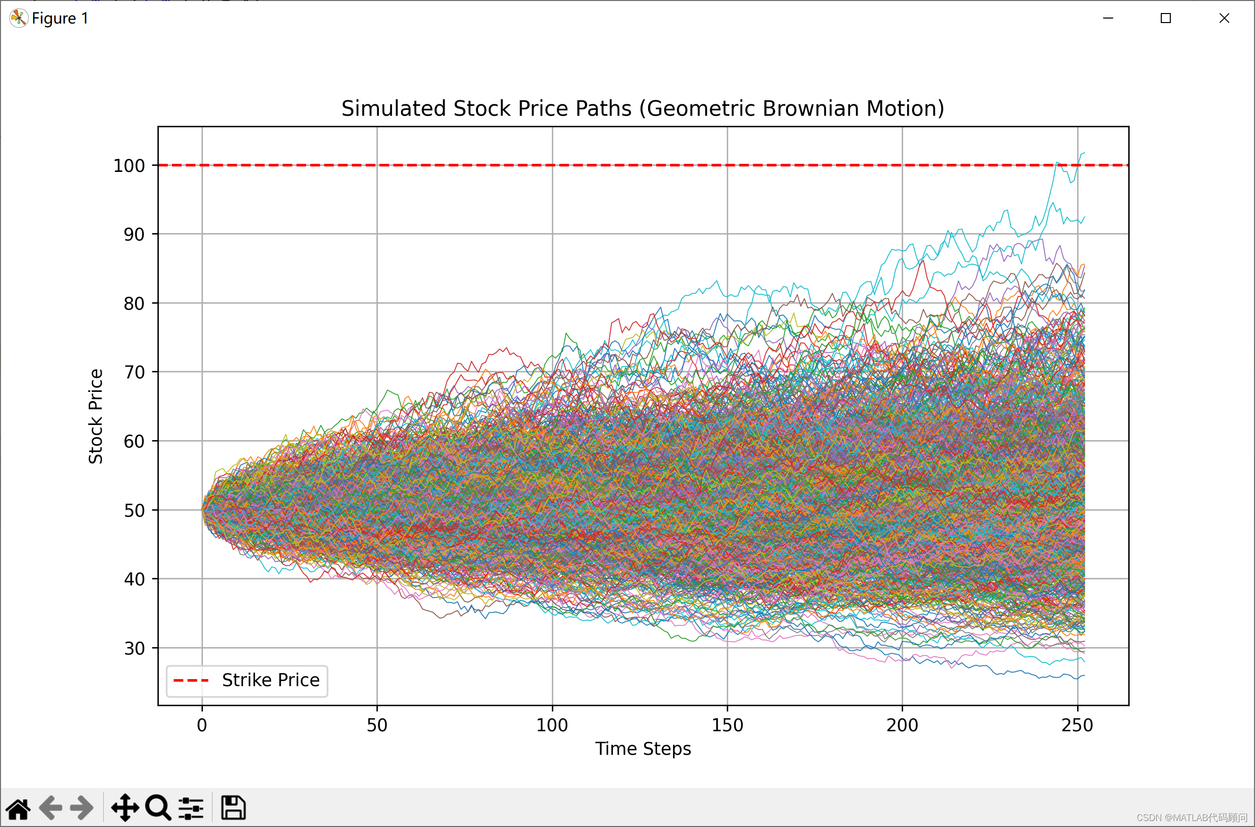
plt.axhline(y=k, color='r', linestyle='--', label='Strike Price')
plt.xlabel('Time Steps')
plt.ylabel('Stock Price')
plt.title('Simulated Stock Price Paths (Geometric Brownian Motion)')
plt.legend()
plt.grid(True)
plt.show()