第T2周：TensorFlow实现彩色图片分类(CIFAR10数据集）,并实现自己的真实图片分类

• 🍨 本文为🔗365天深度学习训练营 中的学习记录博客
• 🍖 原作者：K同学啊

目标：
加载CIFAR-10数据集进行训练，然后能够对彩色图片进行分类
具体实现：
（一）环境：
语言环境：Python 3.10
编 译 器: PyCharm
*框架：*TensorFlow
**（二）具体步骤：
1. 设置使用GPU

# 设置使用GPU  
gpus = tf.config.list_physical_devices("GPU")  
# print(gpus)  
if gpus:  
    gpu0 = gpus[0]  
    tf.config.experimental.set_memory_growth(gpu0, True)  
    tf.config.set_visible_devices([gpu0], "GPU")

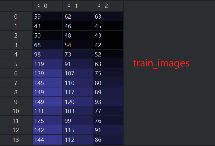
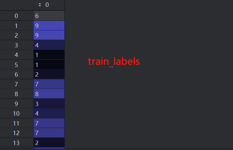
2.导入数据集

# 导入数据集  
(train_images, train_labels), (test_images, test_labels) = datasets.cifar10.load_data()

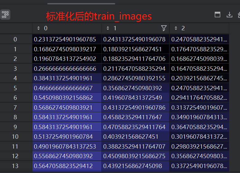
3. 数据标准化

# 数据标准化到0-1区间内  
train_images, test_images = train_images / 255.0, test_images / 255.0  
print(train_images, test_images)

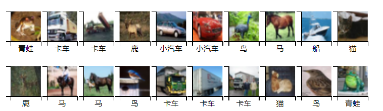
4.可视化数据

# 可视化数据  
class_names = ['飞机', '小汽车', '鸟', '猫', '鹿',  
               '狗', '青蛙', '马', '船', '卡车']
plt.figure(figsize=(20, 10))  
for i in range(20):  
    plt.subplot(5, 10, i+1)  
    plt.xticks([])  
    plt.yticks([])  
    plt.grid(False)  
    plt.imshow(train_images[i], cmap=plt.cm.binary)  
    plt.xlabel(class_names[train_labels[i][0]])  
  
plt.show()

5.构建CNN网络模型

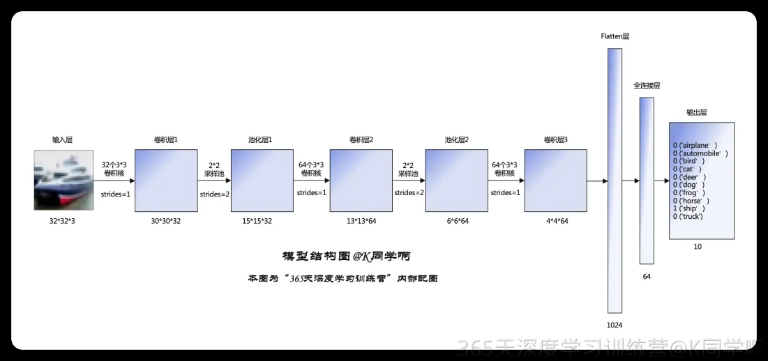
# 构建CNN网络  
model = models.Sequential([  
    layers.Conv2D(32, (3, 3), activation='relu', input_shape=(32, 32, 3)),  
    layers.MaxPooling2D((2, 2)),  
    layers.Conv2D(64, (3, 3), activation='relu'),  
    layers.MaxPooling2D((2, 2)),  
    layers.Conv2D(64, (3, 3), activation='relu'),  
  
    layers.Flatten(),  
    layers.Dense(64, activation='relu'),  
    layers.Dense(10)  
])  
  
print(model.summary())

Model: "sequential"
┌─────────────────────────────────┬────────────────────────┬───────────────┐
│ Layer (type)                    │ Output Shape           │       Param # │
├─────────────────────────────────┼────────────────────────┼───────────────┤
│ conv2d (Conv2D)                 │ (None, 30, 30, 32)     │           896 │
├─────────────────────────────────┼────────────────────────┼───────────────┤
│ max_pooling2d (MaxPooling2D)    │ (None, 15, 15, 32)     │             0 │
├─────────────────────────────────┼────────────────────────┼───────────────┤
│ conv2d_1 (Conv2D)               │ (None, 13, 13, 64)     │        18,496 │
├─────────────────────────────────┼────────────────────────┼───────────────┤
│ max_pooling2d_1 (MaxPooling2D)  │ (None, 6, 6, 64)       │             0 │
├─────────────────────────────────┼────────────────────────┼───────────────┤
│ conv2d_2 (Conv2D)               │ (None, 4, 4, 64)       │        36,928 │
├─────────────────────────────────┼────────────────────────┼───────────────┤
│ flatten (Flatten)               │ (None, 1024)           │             0 │
├─────────────────────────────────┼────────────────────────┼───────────────┤
│ dense (Dense)                   │ (None, 64)             │        65,600 │
├─────────────────────────────────┼────────────────────────┼───────────────┤
│ dense_1 (Dense)                 │ (None, 10)             │           650 │
└─────────────────────────────────┴────────────────────────┴───────────────┘
 Total params: 122,570 (478.79 KB)
 Trainable params: 122,570 (478.79 KB)
 Non-trainable params: 0 (0.00 B)
None

6.编译与训练模型

# 编译模型  
model.compile(optimizer='adam',  
              loss=tf.keras.losses.SparseCategoricalCrossentropy(from_logits=True),  
              metrics=['accuracy'])  
# 训练模型  
history = model.fit(train_images, train_labels, epochs=10, validation_data=(test_images, test_labels))

Epoch 1/10
1563/1563 ━━━━━━━━━━━━━━━━━━━━ 7s 4ms/step - accuracy: 0.3335 - loss: 1.7990 - val_accuracy: 0.5389 - val_loss: 1.2733
Epoch 2/10
1563/1563 ━━━━━━━━━━━━━━━━━━━━ 6s 4ms/step - accuracy: 0.5518 - loss: 1.2573 - val_accuracy: 0.5991 - val_loss: 1.1310
Epoch 3/10
1563/1563 ━━━━━━━━━━━━━━━━━━━━ 6s 4ms/step - accuracy: 0.6235 - loss: 1.0623 - val_accuracy: 0.6547 - val_loss: 0.9888
Epoch 4/10
1563/1563 ━━━━━━━━━━━━━━━━━━━━ 6s 4ms/step - accuracy: 0.6627 - loss: 0.9574 - val_accuracy: 0.6547 - val_loss: 0.9930
Epoch 5/10
1563/1563 ━━━━━━━━━━━━━━━━━━━━ 6s 4ms/step - accuracy: 0.6929 - loss: 0.8715 - val_accuracy: 0.6660 - val_loss: 0.9542
Epoch 6/10
1563/1563 ━━━━━━━━━━━━━━━━━━━━ 6s 4ms/step - accuracy: 0.7174 - loss: 0.8132 - val_accuracy: 0.6943 - val_loss: 0.8771
Epoch 7/10
1563/1563 ━━━━━━━━━━━━━━━━━━━━ 6s 4ms/step - accuracy: 0.7368 - loss: 0.7568 - val_accuracy: 0.6978 - val_loss: 0.8687
Epoch 8/10
1563/1563 ━━━━━━━━━━━━━━━━━━━━ 6s 4ms/step - accuracy: 0.7495 - loss: 0.7141 - val_accuracy: 0.6963 - val_loss: 0.8821
Epoch 9/10
1563/1563 ━━━━━━━━━━━━━━━━━━━━ 6s 4ms/step - accuracy: 0.7682 - loss: 0.6607 - val_accuracy: 0.6795 - val_loss: 0.9167
Epoch 10/10
1563/1563 ━━━━━━━━━━━━━━━━━━━━ 6s 4ms/step - accuracy: 0.7755 - loss: 0.6344 - val_accuracy: 0.7016 - val_loss: 0.8806

7.预测

# 看一下要预测的图片是什么  
plt.imshow(test_images[1])  
plt.show()

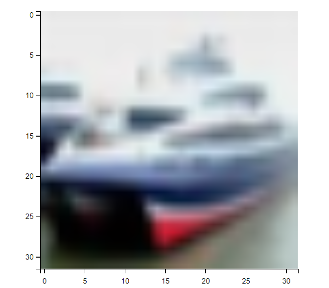
可以看出是一个船。看看模型能否预测准确：

import numpy as np  
pre = model.predict(test_images)  
print(class_names[np.argmax(pre[1])])

预测准确。
8.预测一下我们自己的图片
工程上新创建一个目录data,网上找一张鹿的图片保存在data中：

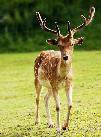
# 预测一下真实照片  
image_path = "data/cat2.jpg"  # 图片存储路径
original_image = tf.io.read_file(image_path, 'r')  
# print(original_image)   # 原始图片数据  
  
# 将原始图片数据转换成tensor格式  
original_image_tensor = tf.io.decode_jpeg(original_image)  
# print(original_image_tensor)    # 打印图片tensor数据  
# print(original_image_tensor.shape)  # 图片形状（750， 500， 3)  
# 根据上面的输入特征（32， 32， 3），因此需要将图片大小改成（32， 32）的。  
original_image_tensor_resize = tf.image.resize(original_image_tensor, [32, 32])  
# print(original_image_tensor_resize.shape)   # resize后的形状  
  
# reshape成（32， 32， 3）  
original_image_tensor_resize_reshape = tf.reshape(original_image_tensor_resize, [-1, 32, 32, 3])  
# 显示图片  
for i in range(3):  
    plt.imshow(original_image_tensor_resize_reshape[0, :, :, i])  
    plt.title(str(i))  
    plt.colorbar()  
    plt.show()  
  
# 再进行标准化到 0-1 区间  
original_image_tensor_resize_reshape_normalize = original_image_tensor_resize_reshape / 255.0  
# print(original_image_tensor_resize_reshape_normalize.shape)  

# 开始预测
import numpy as np  
pre = model.predict(original_image_tensor_resize_reshape_normalize)  
# print(pre)  
# 打印预测结果
print("当前图片预测为: ", class_names[np.argmax(pre[0])])

预测正确。

(三)总结

1. 熟悉各个模型搭建、训练到预测的流程
2. 了解神经网络模型（黑盒子）的细节
3. 并不是每次都能预测正确，对于真实图片的预处理，要怎么样提升准确性，后续研究。
4. 并不是把epochs提高，准确性就提高，继续研究。