【2019/IJCAI】AddGraph: Anomaly Detection in Dynamic Graph Using Attention-based Temporal GCN

文章链接：https://www.ijcai.org/Proceedings/2019/0614.pdf
源码链接：未公布

TL;DR

论文结合GNN提出了动态图中半监督的边异常检测模型 AddGraph，同时考虑了节点的结构，属性和时序特征。对于标签数据不足的问题，在训练过程中采用了 negative sampling 和 margin loss 两个技巧。在两个真实数据集的实验中取得了较好的效果。

Problem Definition

论文中的方法主要用于推荐系统中的异常操作检测，举个例子：异常的用户想自己的物品被推荐，那怎么办，那就找几个人疯狂点自己的东西的同时点那些本身就已经是popular的item，这样就会让自己的物品和popular的有相似的特征等，就会增加这些物品的被推荐的rank。这同时会产生很多新的edge，这些都是异常的edge。如下图所示：

异常模式特征：当异常的用户频繁执行操作时，用户和物品间的边会组成一个 dense subgraph，这种异常的特征模式就需要被检测出来；

Algorithm / Model

AddGraph 的整体架构如下图所示：

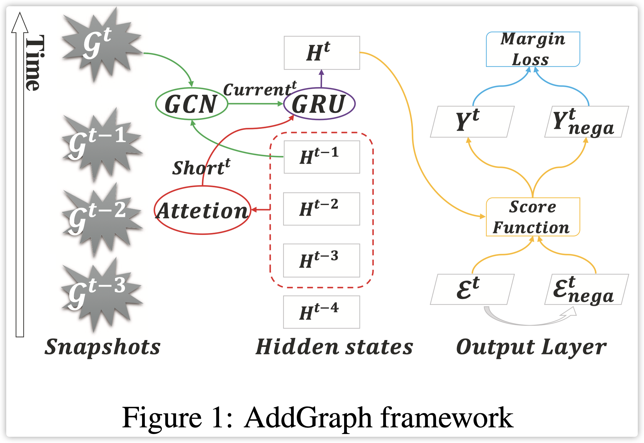
主要分为三部分：

• GCN for content and structural features.
• GRU with attention to combine short-term and long-term states.
• Anomalous score computation for edges.

GCN

给定 $t$ 时刻图流中的一个 snapshot ${\mathcal{G}}^t=\left({\mathcal{V}}^t,{\mathcal{E}}^t\right)$ 、对应的邻接矩阵 $A^t$ 和 $t-1$ 时刻的节点隐含状态矩阵 ${\mathbf{H}}^{t-1}\in {\mathbb{R}}^{n\times d}$，那么当前时刻的节点状态矩阵可以通过 GCN 来更新，
$${\text{ Current }}^t={\mathrm{G}\mathrm{C}\mathrm{N}}_L\left({\mathbf{H}}^{t-1}\right)$$
以上一时刻的节点特征作为当前时刻节点模式的输入，融合了 long-term 特征；对于一个 $L$ 层的GCN，卷积过程如下所示：
$$\begin{array}{rl}{\mathbf{Z}}^{(0)}& ={\mathbf{H}}^{t-1}\\ {\mathbf{Z}}^{(l)}& =\mathrm{Re}LU\left({\hat{\mathbf{A}}}^t{\mathbf{Z}}^{(l-1)}{\mathbf{W}}^{(l-1)}\right)\\ {\text{ Current }}^t& =\mathrm{Re}LU\left({\hat{\mathbf{A}}}^t{\mathbf{Z}}^{(L-1)}{\mathbf{W}}^{(L-1)}\right)\end{array}$$

GRU

为了考虑节点 short-term 的特征，采用了基于上下文注意力模型，以当前的某个时间窗口来编码节点特征，过程如下：
$$\begin{array}{rlr}{\mathbf{C}}_{h,i}^t& =\left[{\mathbf{h}}_i^{t-\omega };\dots ;{\mathbf{h}}_i^{t-1}\right]& {\mathbf{C}}_{h,i}^t\in {\mathbb{R}}^{\omega \times d}\\ {\mathbf{e}}_{h,i}^t& ={\mathbf{r}}^T\tanh \left({\mathbf{Q}}_h{\left({\mathbf{C}}_{h,i}^t\right)}^T\right)& {\mathbf{e}}_{h,i}^t\in {\mathbb{R}}^{\omega }\\ {\mathbf{a}}_{h,i}^t& =\mathrm{softmax}\left({\mathbf{e}}_{h,i}^t\right)& {\mathbf{a}}_{h,i}^t\in {\mathbb{R}}^{\omega }\\ {\mathbf{s}\mathbf{h}\mathbf{o}\mathbf{r}\mathbf{t}}_i^t& ={\left({\mathbf{a}}_{h,i}{\mathbf{C}}_{h,i}^t\right)}^T& {\text{ short }}_i^t\in {\mathbb{R}}^d\end{array}$$
其中 $h_i^t$ 表示节点 $h_i$ 在 $t$ 时刻的特征，$\omega$ 表示时间窗口的大小，${\mathbf{Q}}_h$ 和 $\mathbf{r}$ 是模型需优化的参数；对于所有节点表示成矩阵的计算公司如下：
$${\text{ Short }}^t=\mathrm{C}\mathrm{A}\mathrm{B}\left({\mathbf{H}}^{t-\omega };\dots ;{\mathbf{H}}^{t-1}\right)$$
目前我们得到了包含 long-term 信息的节点特征 ${\text{ Current }}^t$ 和 short-term 信息的节点特征 ${\text{ Short }}^t$，为了考虑时序特征在模型中使用 GRU 来处理这两种特征：
$${\mathbf{H}}^t={\text{ GRU(Current }}^t,\text{ Short }{}^t)$$
具体的前向传播计算公式如下所示：
$$\begin{array}{rl}{\mathbf{P}}^t& =\sigma \left({\mathbf{U}}_P{\text{ Current }}^t+{\mathbf{W}}_P{\text{ Short }}^t+{\mathbf{b}}_P\right)\\ {\mathbf{R}}^t& =\sigma \left({\mathbf{U}}_R{\text{ Current }}^t+{\mathbf{W}}_R{\text{ Short }}^t+{\mathbf{b}}_R\right)\\ {\tilde{\mathbf{H}}}^t& =\tanh \left({\mathbf{U}}_c{\mathbf{C}\mathbf{u}\mathbf{r}\mathbf{r}\mathbf{e}\mathbf{n}\mathbf{t}}^t+{\mathbf{W}}_c\left({\mathbf{R}}^t\odot {\text{ Short }}^t\right)\right)\\ {\mathbf{H}}^t& =\left(1-{\mathbf{P}}^t\right)\odot {\text{ Short }}^t+{\mathbf{P}}^t\odot {\tilde{\mathbf{H}}}^t\end{array}$$
经过上述特征融合的步骤之后，得到的节点特征 ${\mathbf{H}}^t$ 就包含了结构、属性、时序信息；

Anomalous score computation

在编码节点特征 ${\mathbf{H}}^t$ 之后，图中每条边 $(i,j,w)\in {\mathcal{E}}^t$ 的异常概率通过👇的公式进行计算：
$$f(i,j,w)=w\cdot \sigma \left(\beta \cdot \left({\Vert \mathbf{a}\odot {\mathbf{h}}_i+\mathbf{b}\odot {\mathbf{h}}_j\Vert }_2^2-\mu \right)\right)$$
其中 $\sigma (x)=\frac{1}{1+e^x}$ 是sigmoid函数，$\mathbf{a}$ 和 $\mathbf{b}$ 是输出层的参数，$\beta$ 和 $\mu$ 是超参数；

loss function

为了去解决anomaly data不足的情况，我们建立一个模型去描述normal的分布情况，假设训练样本中全部的edge都是normal的，对应每个normal的edge我们产生一个负样本当作anomaly的edge （替换边中的source或者target）。用一个伯努利分布，重新计算了normal边对应两边node的degree，如果这个degree越大则表示越可能是异常的，越小则是正常的；

• marginbased pairwise loss
  度量损失：异常边的评分足够大，正常边的评分足够小；
  L t = min ⁡ ∑ ( i , j , w ) ∈ E t ( i ′ , j ′ , w ) ∉ E t max ⁡ { 0 , γ + f ( i , j , w ) − f ( i ′ , j ′ , w ) } \begin{aligned} \mathcal{L}^{t}=\min & \sum_{(i, j, w) \in \mathcal{E}^{t}\left(i^{\prime}, j^{\prime}, w\right) \notin \mathcal{E}^{t}} \\ & \max \left\{0, \gamma+f(i, j, w)-f\left(i^{\prime}, j^{\prime}, w\right)\right\} \end{aligned} Lt=min​(i,j,w)∈Et(i′,j′,w)∈/​Et∑​max{0,γ+f(i,j,w)−f(i′,j′,w)}​
• L2 regularization loss
  正则损失防止过拟合；
  $$\begin{array}{rl}{\mathcal{L}}_{reg}& =\sum ({\Vert {\mathbf{W}}_1\Vert }_2^2+{\Vert {\mathbf{W}}_2\Vert }_2^2+{\Vert {\mathbf{Q}}_h\Vert }_2^2+\Vert \mathbf{r}{\Vert }_2^2\\ & +{\Vert {\mathbf{U}}_z\Vert }_2^2+{\Vert {\mathbf{W}}_z\Vert }_2^2+{\Vert {\mathbf{b}}_z\Vert }_2^2+{\Vert {\mathbf{U}}_r\Vert }_2^2+{\Vert {\mathbf{W}}_r\Vert }_2^2\\ & +{\Vert {\mathbf{b}}_r\Vert }_2^2+{\Vert {\mathbf{U}}_c\Vert }_2^2+{\Vert {\mathbf{W}}_c\Vert }_2^2+\Vert \mathbf{a}{\Vert }_2^2+\Vert \mathbf{b}{\Vert }_2^2)\end{array}$$
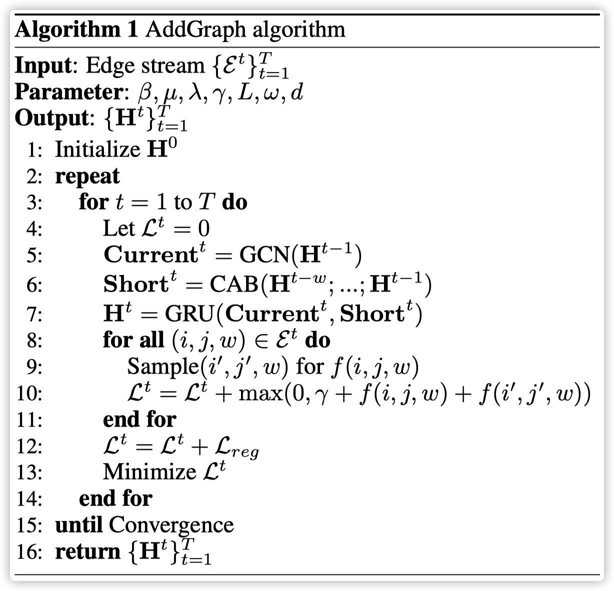
  综上训练的loss 为：
  $$\mathcal{L}={\mathcal{L}}^t+\lambda {\mathcal{L}}_{reg}$$

整体算法伪代码如下：

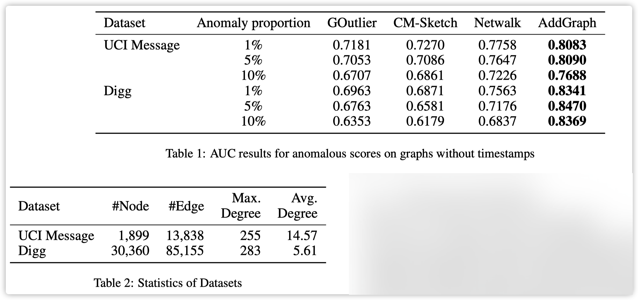
Experiments