PyTorch 中的损失函数总结

最新推荐文章于 2023-04-23 17:21:26 发布

梦家

最新推荐文章于 2023-04-23 17:21:26 发布

阅读量461

点赞数 1

分类专栏： machine learning

本文链接：https://blog.csdn.net/dreamhome_s/article/details/112004810

版权

machine learning 专栏收录该内容

20 篇文章 1 订阅

订阅专栏

原文地址：https://dreamhomes.github.io/posts/202012261041.html

L1Loss

绝对值误差, 主要应用在回归的任务中。

输出维度: (batch_size, 1) # FloatTensor

标签维度: (batch_size, 1) # FloatTensor

实例代码

import torch
from torch import nn
input_data = torch.FloatTensor([[3], [4], [5]])   # batch_size, output
target_data = torch.FloatTensor([[2], [5], [8]])   # batch_size, output 
loss_func = nn.L1Loss()
loss = loss_func(input_data, target_data)
print(loss)  # 1.6667

验证代码

print((abs(3-2) + abs(4-5) + abs(5-8)) / 3)  # 1.6666

MSELoss(L2Loss)

均方误差, 主要应用在回归的任务中

输出维度: (batch_size, 1) # FloatTensor

标签维度: (batch_size, 1) # FloatTensor

实例代码

import torch
from torch import nn
input_data = torch.FloatTensor([[3], [4], [5]])   # batch_size, output
target_data = torch.FloatTensor([[2], [5], [8]])   # batch_size, output 
loss_func = nn.MSELoss()
loss = loss_func(input_data, target_data)
print(loss)   # 3.6667

验证代码

print(((3-2)**2 + (4-5)**2 + (5-8)**2)/3)  # 3.6666666666666665

SmoothL1Loss

损失函数公式为:

$\operatorname{loss}(x, y)=\frac{1}{n} \sum_{i=1}^{n}\left\{\begin{array}{ll} 0.5 *\left(y_{i}-f\left(x_{i}\right)\right)^{2} / \text {beta}, & \text { if }\left|y_{i}-f\left(x_{i}\right)\right|<\text {beta} \\ \left|y_{i}-f\left(x_{i}\right)\right|-0.5 * \text {beta}, & \text {otherwise} \end{array}\right.$

上式的beta是个超参数，不知道咋设置，直接设置为1。仔细观察可以看到，当预测值和ground truth差别较小的时候（绝对值差小于1），其实使用的是L2 Loss；而当差别大的时候，是L1Loss的平移。SooothL1Loss其实是L2Loss和L1Loss的结合，它同时拥有L2 Loss和L1 Loss的部分优点。

实例代码

import torch
from torch import nn
input_data = torch.FloatTensor([[3], [4], [5]])   # batch_size, output
target_data = torch.FloatTensor([[2], [4.1], [8]])   # batch_size, output 
loss_func = nn.SmoothL1Loss()
loss = loss_func(input_data, target_data)
print(loss)   # 输出:1.0017

NLLLoss

负对数似然损失，主要应用在分类任务中。它先通过logSoftmax()，然后把label对应的输出值拿出来，负号去掉，然后平均。

注意: logSoftmax() = log(softmax())

输出维度: (batch_size, class_num) # FloatTensor

标签维度: (batch_size) # LongTensor

实例代码

# 三个样本 进行三分类 使用NLLLoss
import torch
from torch import nn

input = torch.randn(3, 3)
print(input)
# tensor([[ 0.0550, -0.5005, -0.4188],
#         [ 0.7060,  1.1139, -0.0016],
#         [ 0.3008, -0.9968,  0.5147]])
label = torch.LongTensor([0, 2, 1])   # 真实label
loss_func = nn.NLLLoss()
loss = loss_func(temp, label)
print(loss)   # 损失1.6035

验证代码

output = torch.FloatTensor([
        [ 0.0550, -0.5005, -0.4188],
        [ 0.7060,  1.1139, -0.0016],
        [ 0.3008, -0.9968,  0.5147]]
        )

# 1. softmax + log = torch.log_softmax()
sm = nn.Softmax(dim=1)
temp = torch.log(sm(input))
print(temp)  
# tensor([[-0.7868, -1.3423, -1.2607],
#         [-1.0974, -0.6896, -1.8051],
#         [-0.9210, -2.2185, -0.7070]])
# 2. 因为label为[0, 2, 1]  
#    因此第一行取第一个值-0.7868。第二行取第三个值-1.8051，第三行取第二个值-2.2185。然后把负号直接扔掉。 说白的 就是去对数的负值成对应的label  也就是交叉熵。
print((0.7868 + 1.8051 + 2.2185) / 3)   # 输出1.6034666666666666

CrossEntropyLoss

交叉熵，实际上它是由nn.LogSoftmax()和nn.NLLLoss()组成。主要应用在多分类的问题中(二分类也可以用)

输出维度: (batch_size, class_num) # FloatTensor
标签维度: (batch_size,) # LongTensor

实例代码

# 三个样本进行三分类 和上面的数据一样
import torch
from torch import nn
loss_func1 = nn.CrossEntropyLoss()
output = torch.FloatTensor([
        [ 0.0550, -0.5005, -0.4188],
        [ 0.7060,  1.1139, -0.0016],
        [ 0.3008, -0.9968,  0.5147]]
        )

true_label = torch.LongTensor([0, 2, 1])   # 注意这里的label id必须从0开始 不能说label id是1，2，3 必须是0，1，2
loss = loss_func1(output, true_label)
print(loss)  # 输出: 1.6035

目前，发现CrossEntropyLoss和NLLLoss的计算方式是一样的。

BCELoss

BCE Loss就是二分类的交叉熵(它才是严格按照交叉熵的公式去算的，但只针对二分类) BCEloss一般应用在单标签二分类和多标签二分类中。
BCELoss的公式:

$\text {loss } F=-\frac{1}{n} \sum\left(y_{n} \times \operatorname{Inx}_{n}+\left(1-y_{n}\right) \times \operatorname{In}\left(1-x_{n}\right)\right)$

对于单标签二分类模型输出的tensor维度为:(batch_size, 1) # torch.FloatTensor

对于多标签二分类模型输出的tensor维度为(batch_size, class_num) # torch.FloatTensor

标签的维度都是one-hot的形式: (batch_size, one-hot即class_num) # torch.FloatTensor

实例代码

一个样本多标签的分类

import torch
from torch import nn
bce = nn.BCELoss()
output = torch.FloatTensor(
    [
        [ 0.0550, -0.5005, -0.4188],
        [ 0.7060,  1.1139, -0.0016],
        [ 0.3008, -0.9968,  0.5147]
    ]
)
# 注意  输出要经过sigmoid
s = nn.Sigmoid()
output = s(output)
# 假设是一条数据多个标签的分类
label = torch.FloatTensor(
    [
        [1, 0, 1],
        [0, 0, 1],
        [1, 1, 0]
    ]
)
loss = bce(output, label)
print(loss)   # 输出: 0.9013

验证代码

# 1. 模型输出
output = torch.FloatTensor(
    [
        [ 0.0550, -0.5005, -0.4188],
        [ 0.7060,  1.1139, -0.0016],
        [ 0.3008, -0.9968,  0.5147]
    ]
)
# 2. 经过sigmoid
s = nn.Sigmoid()
output = s(output)
# print(output)
# tensor([[0.5137, 0.3774, 0.3968],
#         [0.6695, 0.7529, 0.4996],
#         [0.5746, 0.2696, 0.6259]])
label = torch.FloatTensor(
    [
        [1, 0, 1],
        [0, 0, 1],
        [1, 1, 0]
    ]
)
# 我们根据标签和sigmoid计算出计算
# 第一行
sum_1 = 0
sum_1 += 1 * torch.log(torch.tensor(0.5137)) + (1 - 1) * torch.log(torch.tensor(1 - 0.5137))   # 第一列
sum_1 += 0 * torch.log(torch.tensor(0.3774)) + (1 - 0) * torch.log(torch.tensor(1 - 0.3774))   # 第二列
sum_1 += 1 * torch.log(torch.tensor(0.3968)) + (1 - 1) * torch.log(torch.tensor(1 - 0.3968))   # 第三列
avg_1 = sum_1 / 3
# 第二行
sum_2 = 0
sum_2 += 0 * torch.log(torch.tensor(0.6695)) + (1 - 0) * torch.log(torch.tensor(1 - 0.6695))   # 第一列
sum_2 += 0 * torch.log(torch.tensor(0.7529)) + (1 - 0) * torch.log(torch.tensor(1 - 0.7529))   # 第二列
sum_2 += 1 * torch.log(torch.tensor(0.4996)) + (1 - 1) * torch.log(torch.tensor(1 - 0.4996))   # 第三列
avg_2 = sum_2 / 3
# 第三行
sum_3 = 0
sum_3 += 1 * torch.log(torch.tensor(0.5746)) + (1 - 1) * torch.log(torch.tensor(1 - 0.5746))   # 第一列
sum_3 += 1 * torch.log(torch.tensor(0.2696)) + (1 - 1) * torch.log(torch.tensor(1 - 0.2696))   # 第二列
sum_3 += 0 * torch.log(torch.tensor(0.6259)) + (1 - 0) * torch.log(torch.tensor(1 - 0.6259))   # 第三列
avg_3 = sum_3 / 3

result = -(avg_1 + avg_2 + avg_3) / 3
print(result)   # 输出0.9013

再举个二分类的问题
实例代码

# 两个样本，二分类
import torch
from torch import nn
bce = nn.BCELoss()
output = torch.FloatTensor(
    [
        [ 0.0550, -0.5005],
        [ 0.7060,  1.1139]
    ]
)
# 注意  输出要经过sigmoid
s = nn.Sigmoid()
output = s(output)
# 假设是一条数据多个标签的分类
label = torch.FloatTensor(
    [
        [1, 0],
        [0, 1]
    ]
)
loss = bce(output, label)
print(loss)   # 输出0.6327

验证代码:

output = torch.FloatTensor(
    [
        [ 0.0550, -0.5005],
        [ 0.7060,  1.1139]
    ]
)
# 注意  输出要经过sigmoid
s = nn.Sigmoid()
output = s(output)
# print(output)
# tensor([[0.5137, 0.3774],
#         [0.6695, 0.7529]])
# true_label = [[1, 0], [0, 1]]
sum_1 = 0
sum_1 += 1 * torch.log(torch.tensor(0.5137)) + (1 - 1) * torch.log(torch.tensor(1 - 0.5137))
sum_1 += 0 * torch.log(torch.tensor(0.3774)) + (1 - 0) * torch.log(torch.tensor(1 - 0.3774))
avg_1 = sum_1 / 2

sum_2 = 0
sum_2 += 0 * torch.log(torch.tensor(0.6695)) + (1 - 0) * torch.log(torch.tensor(1 - 0.6695))
sum_2 += 1 * torch.log(torch.tensor(0.7529)) + (1 - 1) * torch.log(torch.tensor(1 - 0.7529))
avg_2 = sum_2 / 2
print(-(avg_1 + avg_2) / 2)  # 输出0.6327

BCEWithLogitsLoss

BCEWithLogitsLoss就是把Sigmoid和BCELoss合成一步。和上面的做法是一样的。如果想用BCE损失，推荐这种，不需要自己写sigmoid那部分。

实例代码

# 用上面那个两个样本进行二分类的数据
import torch
from torch import nn
bce_logit = nn.BCEWithLogitsLoss()
output = torch.FloatTensor(
    [
        [ 0.0550, -0.5005],
        [ 0.7060,  1.1139]
    ]
)   # 未经Sigmoid
label = torch.FloatTensor(
    [
        [1, 0],
        [0, 1]
    ]
)
loss = bce_logit(output, label)
print(loss)   # tensor(0.6327)

Focal Loss

结构介绍

首先声明，这个Focal Loss只是针对二分类问题。

Focal Loss的引入主要是为了解决难易样本数量不平衡（注意，有区别于正负样本数量不平衡）的问题，实际可以使用的范围非常广泛，为了方便解释，还是拿目标检测的应用场景来说明：

单阶段的目标检测器通常会产生高达100k的候选目标，只有极少数是正样本，正负样本数量非常不平衡。我们在计算分类的时候常用的损失——交叉熵的公式如下：

$E=\left\{\begin{array}{ll} -\log (p), & \text { if } y=1 \\ -\log (1-p), & \text { if } y=0 \end{array}\right.$

为了解决正负样本不平衡问题，我们通常会在交叉熵损失的前面加上一个参数α，即:

$E=\left\{\begin{array}{ll} -\alpha \log (p), & \text { if } y=1 \\ -(1-\alpha) \log (1-p), & \text { if } y=0 \end{array}\right.$

但这并不能解决全部问题。根据正、负、难、易，样本一共可以分为以下四类：

$L=\left\{\begin{array}{ll} -(1-p)^{\gamma} \log (p), & \text { if } y=1 \\ -p^{\gamma} \log (1-p), & \text { if } y=0 \end{array}\right.$

尽管 $\alpha$ 平衡了正负样本，但对难易样本的不平衡没有任何帮助。而实际上，目标检测中大量的候选目标易分样本。这些样本的损失很低，但是由于数量极不平衡，易分样本的数量相对来讲太多，最终主导了总的损失。而本文的作者认为，易分样本（即，置信度高的样本）对模型的提升效果非常小，模型应该主要关注那些难分样本（这个假设是有问题的，是GHM的主要改进对象）

Focal Loss就上场了:一个简单的思想：把高置信度§样本的损失再降低一些不就好了吗！

$L=\left\{\begin{array}{ll} -(1-p)^{\gamma} \log (p), & \text { if } y=1 \\ -p^{\gamma} \log (1-p), & \text { if } y=0 \end{array}\right.$

举个例, $\gamma$ 取2时，如果p = 0.968 , (1-0.968)^2≈0.001 ，损失衰减了1000倍！

Focal Loss的最终形式结合了上面的公式2解决了正负样本的不平衡，公式3解决了难易样本的不平衡，将公式 2 与 3 结合使用，同时解决正负难易2个问题！

最终的Focal Loss形式如下：

$L=\left\{\begin{array}{ll} -\alpha(1-p)^{\gamma} \log (p), & \text { if } y=1 \\ -(1-\alpha) p^{\gamma} \log (1-p), & \text { if } y=0 \end{array}\right.$

实验表明: $\gamma$ 取2, $\alpha$ 取0.25的时候效果更佳。

Focal Loss的代码实现

import torch
import torch.nn.functional as F


def reduce_loss(loss, reduction):
    reduction_enum = F._Reduction.get_enum(reduction)
    # none: 0, elementwise_mean:1, sum: 2
    if reduction_enum == 0:
        return loss
    elif reduction_enum == 1:
        return loss.mean()
    elif reduction_enum == 2:
        return loss.sum()


def weight_reduce_loss(loss, weight=None, reduction='mean', avg_factor=None):
    if weight is not None:
        loss = loss * weight

    if avg_factor is None:
        loss = reduce_loss(loss, reduction)
    else:
        # if reduction is mean, then average the loss by avg_factor
        if reduction == 'mean':
            loss = loss.sum() / avg_factor
        # if reduction is 'none', then do nothing, otherwise raise an error
        elif reduction != 'none':
            raise ValueError('avg_factor can not be used with reduction="sum"')
    return loss


def py_sigmoid_focal_loss(pred, target, weight=None, gamma=2.0, alpha=0.25, reduction='mean', avg_factor=None):
    # 注意 输入的pred不需要经过sigmoid
    pred_sigmoid = pred.sigmoid()
    target = target.type_as(pred)
    pt = (1 - pred_sigmoid) * target + pred_sigmoid * (1 - target)
    focal_weight = (alpha * target + (1 - alpha) *
                    (1 - target)) * pt.pow(gamma)
    # 下面求交叉熵的这个函数 对pred进行了sigmoid
    loss = F.binary_cross_entropy_with_logits(
        pred, target, reduction='none') * focal_weight
    # print(loss)
    '''输出
    tensor([[0.0394, 0.0506],
        [0.3722, 0.0043]])
        '''
    loss = weight_reduce_loss(loss, weight, reduction, avg_factor)
    return loss


if __name__ == '__main__':
    output = torch.FloatTensor(
        [
            [0.0550, -0.5005],
            [0.7060, 1.1139]
        ]
    )
    label = torch.FloatTensor(
        [
            [1, 0],
            [0, 1]
        ]
    )
    loss = py_sigmoid_focal_loss(output, label)
    print(loss)

GHM Loss

结构介绍

Focal Loss存在什么问题呢？

首先，让模型过多关注那些特别难分的样本肯定是存在问题的，样本中有离群点（outliers），可能模型已经收敛了但是这些离群点还是会被判断错误，让模型去关注这样的样本，怎么可能是最好的呢？

其次，α和γ取值全凭实验得出，且α和γ要联合起来一起实验才行(也就是说,α和γ的取值会相互影响)。

Focal Loss是从置信度p的角度入手衰减loss, 而GHM是一定范围内置信度p的样本数量的角度衰减loss。

文章首先定义了一个梯度模长g:

$g=\left|p-p^{*}\right|=\left\{\begin{array}{ll} 1-p, & \text { if } p^{*}=1 \\ p, & \text { if } p^{*}=0 \end{array}\right.$

其中， $p$ 是模型预测的概率， $p^*$ 是ground-truth的标签， $p^*$ 的取值为0或1。 $g$ 正比于检测的难易程度， $g$ 越大则检测难道越大.

至于为什么叫梯度模长，因为g是从交叉熵损失求梯度得来的:

$L_{C E}=\left\{\begin{array}{ll} -\log (p), & \text { if } p^{*}=1 \\ -\log (1-p), & \text { if } p^{*}=0 \end{array}\right.$

看下图梯度模长与样本数量的关系:

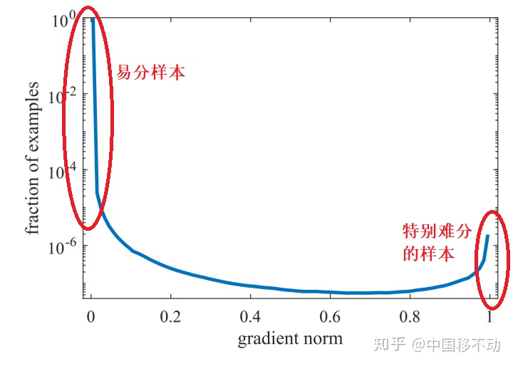
可以看到，梯度模长接近于0的样本数量最多，随着梯度模长的增长，样本数量迅速减少，但是在梯度模长接近于1时，样本数量也挺多。

GHM的想法是，我们确实不应该过多关注易分样本，但是特别难分的样本（outliers，离群点）也不该关注啊！

这些离群点的梯度模长d要比一般的样本大很多，如果模型被迫去关注这些样本，反而有可能降低模型的准确度！况且，这些样本的数量也很多！

那怎么同时衰减易分样本和特别难分的样本呢?太简单了，谁的数量多衰减谁呗！那怎么衰减数量多的呢？简单啊，定义一个变量，让这个变量能衡量出一定梯度范围内的样本数量——这不就是物理上密度的概念吗？

于是，作者定义了梯度密度 GD(g) ——本文最重要的公式：

$D(g)=\frac{1}{l_{\epsilon}(g)} \sum_{k=1}^{N} \delta_{\epsilon}\left(g_{k}, g\right)$

其中δ_ϵ(g_k, g)表明了样本1-N中，梯度模长分布在(g-ϵ/2, g+ϵ/2)范围内的样本个数，l_ϵ(g)代表了(g-ϵ/2, g+ϵ/2)区间的长度。因此梯度密度 GD(g) 的物理含义是：单位梯度模长g部分的样本个数。

加下来就简单了，对于每个样本，把交叉熵CE x 该样本梯度密度的倒数即可！

因此，用于分类的GHM损失函数:

$L_{G H M-C}=\sum_{i=1}^{N} \frac{L_{C E}\left(p_{i}, p_{i}^{*}\right)}{G D\left(g_{i}\right)}$

$N$ 是总的样本数量。

梯度密度的详细计算过程如下:
首先，把梯度模长范围划分成10个区域，这里要求输入必须经过sigmoid计算，这样梯度模长的范围就限制在0~1之间：

class GHMC(nn.Module):
    def __init__(self, bins=10, ......):
        self.bins = bins
        edges = torch.arange(bins + 1).float() / bins

edges是每个区域的边界，有了边界就很容易计算出梯度模长落入哪个区间内。

然后根据网络输出pred和ground true计算loss：

注意，不管是Focal Loss还是GHM其实都是对不同样本赋予不同的权重，所以该代码前面计算的都是样本权重，最后计算GHM Loss就是调用了Pytorch自带的binary_cross_entropy_with_logits，将样本权重填进去。

看看抑制的效果吧。

同样，对于回归损失:

$L_{G H M-R}=\sum_{i=1}^{N} \frac{A S L_{1} d_{i}}{G D\left(g r_{i}\right)}$

其中 ASL₁为修正的smooth L1 Loss

GHM-Loss的代码实现

"""
# -*- coding: utf-8 -*-
# @File    : temp2.py
# @Time    : 2020/12/30 3:03 上午
# @Author  : xiaolu
# @Email   : luxiaonlp@163.com
# @Software: PyCharm
"""
import torch
from torch import nn
import torch.nn.functional as F


class GHM_Loss(nn.Module):
    def __init__(self, bins, alpha):
        super(GHM_Loss, self).__init__()
        self._bins = bins
        self._alpha = alpha
        self._last_bin_count = None

    def _g2bin(self, g):
        return torch.floor(g * (self._bins - 0.0001)).long()

    def _custom_loss(self, x, target, weight):
        raise NotImplementedError

    def _custom_loss_grad(self, x, target):
        raise NotImplementedError

    def forward(self, x, target):
        g = torch.abs(self._custom_loss_grad(x, target)).detach()

        bin_idx = self._g2bin(g)

        bin_count = torch.zeros((self._bins))
        for i in range(self._bins):
            bin_count[i] = (bin_idx == i).sum().item()

        N = (x.size(0) * x.size(1))

        if self._last_bin_count is None:
            self._last_bin_count = bin_count
        else:
            bin_count = self._alpha * self._last_bin_count + (1 - self._alpha) * bin_count
            self._last_bin_count = bin_count

        nonempty_bins = (bin_count > 0).sum().item()

        gd = bin_count * nonempty_bins
        gd = torch.clamp(gd, min=0.0001)
        beta = N / gd

        return self._custom_loss(x, target, beta[bin_idx])


class GHMC_Loss(GHM_Loss):
    # 分类损失
    def __init__(self, bins, alpha):
        super(GHMC_Loss, self).__init__(bins, alpha)

    def _custom_loss(self, x, target, weight):
        return F.binary_cross_entropy_with_logits(x, target, weight=weight)

    def _custom_loss_grad(self, x, target):
        return torch.sigmoid(x).detach() - target


class GHMR_Loss(GHM_Loss):
    # 回归损失
    def __init__(self, bins, alpha, mu):
        super(GHMR_Loss, self).__init__(bins, alpha)
        self._mu = mu

    def _custom_loss(self, x, target, weight):
        d = x - target
        mu = self._mu
        loss = torch.sqrt(d * d + mu * mu) - mu
        N = x.size(0) * x.size(1)
        return (loss * weight).sum() / N

    def _custom_loss_grad(self, x, target):
        d = x - target
        mu = self._mu
        return d / torch.sqrt(d * d + mu * mu)


if __name__ == '__main__':
    # 这个损失函数不需要自己进行sigmoid
    output = torch.FloatTensor(
        [
            [0.0550, -0.5005],
            [0.7060, 1.1139]
        ]
    )
    label = torch.FloatTensor(
        [
            [1, 0],
            [0, 1]
        ]
    )
    loss_func = GHMC_Loss(bins=10, alpha=0.75)
    loss = loss_func(output, label)
    print(loss)

参考原文：https://zhuanlan.zhihu.com/p/340585479

联系作者

梦家

关注

1
点赞
踩
7

收藏

觉得还不错? 一键收藏
1
评论
PyTorch 中的损失函数总结

原文地址：https://dreamhomes.github.io/posts/202012261041.html文章目录原文地址：[https://dreamhomes.github.io/posts/202012261041.html](https://dreamhomes.github.io/posts/202012261041.html)L1Loss实例代码验证代码MSELoss(L2Loss)实例代码验证代码SmoothL1Loss实例代码NLLLoss实例代码验证代码CrossEntropy.
复制链接

扫一扫