解锁视觉-文本双编码：CLIP类似模型的多GPU训练

最新推荐文章于 2025-02-28 11:52:57 发布

109702008

最新推荐文章于 2025-02-28 11:52:57 发布

阅读量1.7k

点赞数 29

分类专栏： # ROCm 文章标签：人工智能学习

本文链接：https://blog.csdn.net/eidolon_foot/article/details/143663335

版权

ROCm 专栏收录该内容

122 篇文章

订阅专栏

Unlocking Vision-Text Dual-Encoding: Multi-GPU Training of a CLIP-Like Model ROCm Blogs

2024年4月24日，由Sean Song撰写。

在本博客中，我们将构建一个类似CLIP的视觉-文本双编码器模型，并在AMD GPU上使用ROCm对其进行微调，使用COCO数据集。这项工作受到CLIP原理和Hugging Face 示例的启发。我们的目标是联合训练一个视觉编码器和一个文本编码器，将图像及其描述的表示投射到相同的嵌入空间中，使文本嵌入位于描述其图像的嵌入附近。在训练过程中，目标是最大化批次内图像和文本对嵌入的相似性，同时最小化错误对的嵌入相似性。该模型通过学习一个多模态嵌入空间来实现这一点。使用对称交叉熵损失优化这些相似性分数。

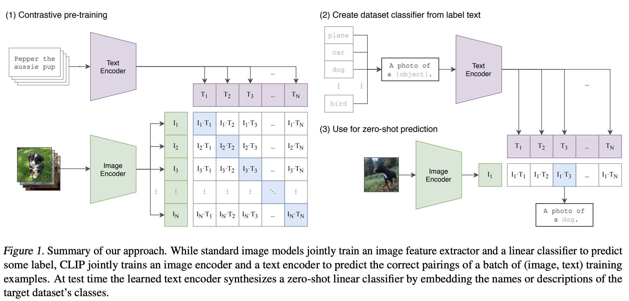
png

图片来源：从自然语言监督中学习可迁移的视觉模型。

视觉-文本双编码器模型可以应用于广泛的下游视觉和语言任务，如图像分类、目标检测、图像描述、视觉问答等。参考我们之前的与CLIP互动博客，了解如何使用预训练的CLIP模型来计算图像和文本之间的相似性，以实现零样本图像分类。
您可以在vision-text-dual-encoding找到本博客中使用的完整代码。

配置

本演示是在以下设置下创建的。有关全面的支持细节，请参阅 ROCm 文档.

硬件和操作系统:
- 支持的 AMD GPU
- Ubuntu 22.04.3 LTS
软件:
- ROCm 5.7.0+
- PyTorch 2.0+

1. 入门

安装所需的库。

!pip install datasets accelerate matplotlib -U

建议从源代码安装 Transformers。

%%bash
git clone https://github.com/huggingface/transformers
cd transformers
pip install -e .

检查系统上 GPU 的可用性。

!rocm-smi

==================== ROCm System Management Interface =========================
========================= Concise Info ===================================
    GPU  Temp (DieEdge)  AvgPwr  SCLK    MCLK     Fan  Perf  PwrCap  VRAM%  GPU%  
    0    39.0c           41.0W   800Mhz  1600Mhz  0%   auto  300.0W    0%   0%    
    1    42.0c           43.0W   800Mhz  1600Mhz  0%   auto  300.0W    0%   0%    
    2    41.0c           43.0W   800Mhz  1600Mhz  0%   auto  300.0W    0%   0%    
    3    41.0c           40.0W   800Mhz  1600Mhz  0%   auto  300.0W    0%   0%    
    4    41.0c           44.0W   800Mhz  1600Mhz  0%   auto  300.0W    0%   0%    
    5    40.0c           42.0W   800Mhz  1600Mhz  0%   auto  300.0W    0%   0%    
    6    37.0c           43.0W   800Mhz  1600Mhz  0%   auto  300.0W    0%   0%    
    7    40.0c           43.0W   800Mhz  1600Mhz  0%   auto  300.0W    0%   0%    
    ====================================================================================
=================== End of ROCm SMI Log ================================

2. 下载 COCO 数据集

以下示例使用了 COCO 数据集 (2017) 通过自定义数据集脚本，要求用户在训练前手动下载 COCO 数据集。下载时间取决于网络速度。根据我们的经验，从终端启动大约需要 7 分钟。从 Jupyter notebook 单元格下载时间会更长。

%%bash
mkdir data
cd data
wget http://images.cocodataset.org/zips/train2017.zip
wget http://images.cocodataset.org/zips/val2017.zip
wget http://images.cocodataset.org/zips/test2017.zip
wget http://images.cocodataset.org/annotations/annotations_trainval2017.zip
wget http://images.cocodataset.org/annotations/image_info_test2017.zip
cd ..

一旦您手动下载了 COCO 数据集，请使用提供的脚本加载它(ydshieh/coc_dataset_script).

import os
import datasets

COCO_DIR = os.path.join(os.getcwd(), "data")
ds = datasets.load_dataset("ydshieh/coco_dataset_script", "2017", data_dir=COCO_DIR)
print(ds["train"])

    Dataset({
        features: ['image_id', 'caption_id', 'caption', 'height', 'width', 'file_name', 'coco_url', 'image_path'],
        num_rows: 591753
    })

每个数据样本由上述八个字段组成。在对比学习的背景下，当图像和字幕来自同一个样本时，它们成对作为正例；当它们不匹配并来自不同样本时，则作为负例。以下是训练数据集中的四个样本。

import matplotlib.pyplot as plt
from PIL import Image
import requests

f, axarr = plt.subplots(2,2, figsize=(8,8))
plt.subplots_adjust(hspace=-0.3, wspace=1.2)
for index in range(4):
    image = Image.open(requests.get(ds["train"][index]['coco_url'], stream=True).raw).resize((128,128)).convert("RGB")
    caption = ds["train"][index]['caption']
    axarr[index//2,index%2].imshow(image)
    axarr[index//2,index%2].title.set_text(caption)
    axarr[index//2,index%2].title.set_size(9) 
    axarr[index//2,index%2].set_xticks([])
    axarr[index//2,index%2].set_yticks([])

png

3. 创建一个类似 CLIP 的视觉-文本双编码器模型

我们使用 VisionTextDualEncoderModel 来构建类似 CLIP 模型的视觉-文本双编码器模型。这个 VisionTextDualEncoderModel 类可以用于初始化一个具有任何预训练视觉自动编码模型作为视觉编码器和预训练语言模型作为文本编码器的视觉-文本双编码器模型。在我们的案例中，我们使用 openai/clip-vit-base-patch32 和 roberta-base 分别作为视觉编码器和文本编码器。

from transformers import (
    VisionTextDualEncoderModel,
    VisionTextDualEncoderProcessor,
    AutoTokenizer,
    AutoImageProcessor
)

model = VisionTextDualEncoderModel.from_vision_text_pretrained(
    "openai/clip-vit-base-patch32", "roberta-base"
)

# 从文本和视觉编码器中获取分词器和图像处理器 
tokenizer = AutoTokenizer.from_pretrained("roberta-base")
image_processor = AutoImageProcessor.from_pretrained("openai/clip-vit-base-patch32")
processor = VisionTextDualEncoderProcessor(image_processor, tokenizer)

# 保存模型和处理器
model.save_pretrained("clip-roberta")
processor.save_pretrained("clip-roberta")
# 检查模型  
print(model)

输出:

    VisionTextDualEncoderModel(
      (vision_model): CLIPVisionModel(
        (vision_model): CLIPVisionTransformer(
          (embeddings): CLIPVisionEmbeddings(
            (patch_embedding): Conv2d(3, 768, kernel_size=(32, 32), stride=(32, 32), bias=False)
            (position_embedding): Embedding(50, 768)
          )
          (pre_layrnorm): LayerNorm((768,), eps=1e-05, elementwise_affine=True)
          (encoder): CLIPEncoder(
            (layers): ModuleList(
              (0-11): 12 x CLIPEncoderLayer(
                (self_attn): CLIPAttention(
                  (k_proj): Linear(in_features=768, out_features=768, bias=True)
                  (v_proj): Linear(in_features=768, out_features=768, bias=True)
                  (q_proj): Linear(in_features=768, out_features=768, bias=True)
                  (out_proj): Linear(in_features=768, out_features=768, bias=True)
                )
                (layer_norm1): LayerNorm((768,), eps=1e-05, elementwise_affine=True)
                (mlp): CLIPMLP(
                  (activation_fn): QuickGELUActivation()
                  (fc1): Linear(in_features=768, out_features=3072, bias=True)
                  (fc2): Linear(in_features=3072, out_features=768, bias=True)
                )
                (layer_norm2): LayerNorm((768,), eps=1e-05, elementwise_affine=True)
              )
            )
          )
          (post_layernorm): LayerNorm((768,), eps=1e-05, elementwise_affine=True)
        )
      )
      (text_model): RobertaModel(
        (embeddings): RobertaEmbeddings(
          (word_embeddings): Embedding(50265, 768, padding_idx=1)
          (position_embeddings): Embedding(514, 768, padding_idx=1)
          (token_type_embeddings): Embedding(1, 768)
          (LayerNorm): LayerNorm((768,), eps=1e-05, elementwise_affine=True)
          (dropout): Dropout(p=0.1, inplace=False)
        )
        (encoder): RobertaEncoder(
          (layer): ModuleList(
            (0-11): 12 x RobertaLayer(
              (attention): RobertaAttention(
                (self): RobertaSelfAttention(
                  (query): Linear(in_features=768, out_features=768, bias=True)
                  (key): Linear(in_features=768, out_features=768, bias=True)
                  (value): Linear(in_features=768, out_features=768, bias=True)
                  (dropout): Dropout(p=0.1, inplace=False)
                )
                (output): RobertaSelfOutput(
                  (dense): Linear(in_features=768, out_features=768, bias=True)
                  (LayerNorm): LayerNorm((768,), eps=1e-05, elementwise_affine=True)
                  (dropout): Dropout(p=0.1, inplace=False)
                )
              )
              (intermediate): RobertaIntermediate(
                (dense): Linear(in_features=768, out_features=3072, bias=True)
                (intermediate_act_fn): GELUActivation()
              )
              (output): RobertaOutput(
                (dense): Linear(in_features=3072, out_features=768, bias=True)
                (LayerNorm): LayerNorm((768,), eps=1e-05, elementwise_affine=True)
                (dropout): Dropout(p=0.1, inplace=False)
              )
            )
          )
        )
        (pooler): RobertaPooler(
          (dense): Linear(in_features=768, out_features=768, bias=True)
          (activation): Tanh()
        )
      )
      (visual_projection): Linear(in_features=768, out_features=512, bias=False)
      (text_projection): Linear(in_features=768, out_features=512, bias=False)
    )

文本编码器和视觉编码器都加载了预训练权重。由于投影层是随机初始化的，并且我们没有联合训练这两个编码器，直接使用这个模型来计算图像和文本之间的相似性不会产生令人满意的结果。为了探索这一局限性，让我们进行一个快速测试。为了方便参考，我们将这个构建的模型命名为 clip-roberta。

3.1. 为clip-roberta创建测试数据

首先，准备包括六张图片和六个文字描述的测试数据。

urls = [
    "http://images.cocodataset.org/val2017/000000039769.jpg",
    "https://farm3.staticflickr.com/2674/5850229113_4fe05d5265_z.jpg",
    "http://farm6.staticflickr.com/5250/5255601114_e6bd308f74_z.jpg",
    "http://farm4.staticflickr.com/3389/3251688524_b35eaf2acd_z.jpg",
    "https://m.media-amazon.com/images/W/MEDIAX_849526-T1/images/I/51hDgswvNqL._AC_.jpg",
    "http://farm1.staticflickr.com/62/202534637_2dbb3071e5_z.jpg",
]
images = [Image.open(requests.get(url, stream=True).raw) for url in urls]

f, axarr = plt.subplots(2,3)
axarr[0,0].imshow(images[0])
axarr[0,1].imshow(images[1])
axarr[0,2].imshow(images[2])
axarr[1,0].imshow(images[3])
axarr[1,1].imshow(images[4])
axarr[1,2].imshow(images[5])

texts = ["a photo of a cat", "a photo of a dog", "a photo of an airplane", "a photo of a horse", "a photo of a tree", "a photo of a bench"]

png

3.2. 处理图像和文本并将其输入clip-roberta模型

# 推断
inputs = processor(
    text=texts, images=images, return_tensors="pt", padding=True
)
outputs = model(**inputs)
logits_per_image = outputs.logits_per_image  # this is the image-text similarity score
print(logits_per_image)
probs = logits_per_image.softmax(dim=1)  # we can take the softmax to get the label probabilities

输出:

    tensor([[ 0.4270,  0.4314,  0.4330,  0.4296,  0.4369,  0.4647],
            [ 1.2838,  1.2888,  1.2693,  1.2823,  1.2885,  1.2793],
            [ 0.9680,  0.9829,  0.9737,  0.9589,  0.9696,  0.9837],
            [ 0.4647,  0.4655,  0.4695,  0.4623,  0.4461,  0.4612],
            [-0.1244, -0.1225, -0.1151, -0.1315, -0.1097, -0.1017],
            [ 0.2710,  0.2707,  0.2837,  0.2689,  0.2669,  0.2833]],
           grad_fn=<PermuteBackward0>)

3.3. 可视化相似度分数

我们可以使用热图可视化图像和文本之间的相似度分数。分数越高，文本和图像特征越相似。

count = len(texts)
similarity = probs.detach().numpy()
plt.figure(figsize=(5, 9))
plt.imshow(similarity, vmin=0.1, vmax=0.3)
plt.yticks(range(count), texts, fontsize=10)
plt.xticks([])
for i, image in enumerate(images):
    plt.imshow(image, extent=(i - 0.5, i + 0.5, -1.6, -0.6), origin="lower")
for x in range(similarity.shape[1]):
    for y in range(similarity.shape[0]):
        plt.text(x, y, f"{similarity[y, x]:.3f}", ha="center", va="center", size=10)

for side in ["left", "top", "right", "bottom"]:
  plt.gca().spines[side].set_visible(False)

plt.xlim([-0.5, count - 0.5])
plt.ylim([count-0.5, -1.8])

plt.title("Similarity between text and image features", size=10)

png

如前所述，由于投影层是随机初始化的，并且视觉和文本编码器是分开训练的，因此模型当前无法提供准确的结果。它倾向于为每对图像和文本分配相似的分数，而不是准确地分别评估它们。这是预期的结果。下一步涉及对模型进行联合训练，然后使用相同的测试重新评估其性能。

4. 利用COCO数据集训练模型

你可以很方便地使用 Weights & Biases. 来记录和监控训练过程。要使用Weights & Biases，先安装`wandb`包：

!pip install wandb

接着导入并登录wandb:

import wandb
wandb.login()

# 如果你不想使用wandb，用以下两行代码替代上面的代码
# import os
# os.environ["WANDB_DISABLED"] = "true"

最后，我们准备使用 run_clip.py 脚本训练我们的 clip-roberta 模型。在训练中，我们使用 Hugging Face 的 Trainer 和TrainingArguments ，它们提供了一种便捷的方法来根据需求定制训练过程。我们将模型训练5个epochs，并每500步保存一次检查点。你可以提高这个配置以减少保存所带来的开销。以下是相关的设定：

%%bash
torchrun \
    --nproc_per_node 8 ./run_clip.py \
    --output_dir ./clip-roberta-finetuned \
    --model_name_or_path ./clip-roberta \
    --data_dir $PWD/data \
    --dataset_name ydshieh/coco_dataset_script \
    --dataset_config_name=2017 \
    --image_column image_path \
    --caption_column caption \
    --remove_unused_columns=False \
    --do_train  --do_eval\
    --per_device_train_batch_size="64" \
    --per_device_eval_batch_size="64" \
    --learning_rate="5e-5" --warmup_steps="0" --weight_decay 0.1 \
    --num_train_epochs=5 \
    --overwrite_output_dir

如果你的系统配备了多个GPU，可以通过在`nproc_per_node`中指定可用GPU的数量来加速训练过程（以下训练使用8个GPU）。下表展示了使用不同数量的GPU（AMD Instinct MI210）时的训练运行时间:

Number of GPUs	1	2	4	8
Train Runtime (hours)	7.8	5.2	2.5	1.3

在训练完成后，模型 clip-roberta-finetuned 将会被保存。你可以在训练开始时找到类似的输出。点击提供的链接可以访问并追踪训练指标，例如训练损失。

wandb: ⭐️ 查看项目 https://wandb.ai/your-account/huggingface
wandb: 🚀 查看项目 https://wandb.ai/your-account/huggingface/runs/0q98bm04 \

png

从之前的训练损失图表中，我们观察到损失一致下降，这符合我们的预期。然而，本博客的目的不是深入探讨所有可能的训练配置以获得最佳模型，而是聚焦于利用AMD多GPU的强大功能来释放视觉-文本双编码的潜力。

接下来，我们将对微调后的模型 (clip-roberta-finetuned) 进行测试，以评估其准确分类`clip-roberta`难以处理的图像的能力。

5. 测试微调后的模型

加载 clip-roberta-finetuned 模型并使用之前用过的测试数据进行测试。

model = VisionTextDualEncoderModel.from_pretrained(
    "./clip-roberta-finetuned"
)
# 从文本和视觉编码器中获取 tokenizer 和图像处理器 
tokenizer = AutoTokenizer.from_pretrained("./clip-roberta-finetuned")
image_processor = AutoImageProcessor.from_pretrained("./clip-roberta-finetuned")
processor = VisionTextDualEncoderProcessor(image_processor, tokenizer)

# 推理
outputs = model(**inputs)
logits_per_image = outputs.logits_per_image  # 这是图像-文本的相似度得分
probs = logits_per_image.softmax(dim=1)  # 我们可以通过 softmax 获取标签的概率 probabilities
print(probs)

输出:

    tensor([[9.8811e-01, 1.6277e-03, 9.7421e-04, 4.5114e-03, 3.1330e-03, 1.6449e-03],
            [9.7203e-04, 9.9060e-01, 3.4517e-04, 5.8935e-03, 1.9453e-03, 2.4285e-04],
            [1.3150e-05, 3.2590e-05, 9.9988e-01, 2.8037e-05, 1.6928e-05, 3.3404e-05],
            [5.4424e-03, 1.6018e-02, 5.6439e-04, 8.7959e-01, 9.7941e-02, 4.4352e-04],
            [9.0918e-07, 3.3684e-06, 8.4072e-07, 1.0356e-05, 9.9989e-01, 9.4088e-05],
            [6.3964e-05, 1.7778e-05, 9.8011e-06, 4.8208e-04, 5.2074e-05, 9.9937e-01]],
           grad_fn=<SoftmaxBackward0>)

最后，我们将展示结果，看到每幅图像都已被 clip-roberta-finetuned 模型正确分类。这一结果成功展示了我们训练的有效性。

count = len(texts)
similarity = probs.detach().numpy()
plt.figure(figsize=(5, 9))
plt.imshow(similarity, vmin=0.1, vmax=0.3)
plt.yticks(range(count), texts, fontsize=10)
plt.xticks([])
for i, image in enumerate(images):
    plt.imshow(image, extent=(i - 0.5, i + 0.5, -1.6, -0.6), origin="lower")
for x in range(similarity.shape[1]):
    for y in range(similarity.shape[0]):
        plt.text(x, y, f"{similarity[y, x]:.3f}", ha="center", va="center", size=10)

for side in ["left", "top", "right", "bottom"]:
  plt.gca().spines[side].set_visible(False)

plt.xlim([-0.5, count - 0.5])
plt.ylim([count-0.5, -1.8])

plt.title("Similarity between text and image features", size=10)

png