PyTorch 深度学习（一）

最新推荐文章于 2022-01-20 00:40:59 发布

shchojj

最新推荐文章于 2022-01-20 00:40:59 发布

阅读量350

点赞数

分类专栏： pytorch

原文链接：https://pytorch.apachecn.org/docs/1.7/02.html

版权

pytorch 专栏收录该内容

11 篇文章 1 订阅

订阅专栏

https://pytorch.apachecn.org/docs/1.7/02.html

最近没有正经看过源码，在回溯一下，以免忘记。

pytorch有自动微分机制。

张量

可以理解为多维数组

张量初始化

import torch
import numpy as np
#****************直接生成张量****************#
data = [[1,2],[3,4]]
x_data = torch.tensor(data)
#***************numpy生成张量****************#
np_array = np.array(data)
x_np = torch.from_numpy(np_array)
#****************张量生成张量****************#
x_ones = torch.ones_like(x_data) # 保留x_data属性
x_rand = torch.rand_like(x_data, dtype=torch.float) # 设置x_data数据类型
print(f"Ones Tensor: \n {x_ones} \n")
print(f"Random Tensor: \n {x_rand} \n")
#**************生成指定维度张量**************#
shape = (2,3,)
rand_tensor = torch.rand(shape)
ones_tensor = torch.ones(shape)
zeros_tensor = torch.zeros(shape)
print(f"Random Tensor: \n {rand_tensor} \n")
print(f"Ones Tensor: \n {ones_tensor} \n")
print(f"Zeros Tensor: \n {zeros_tensor}")
#******************张量属性******************#
tensor = torch.rand(3,4)
print(f"Shape of tensor: {tensor.shape}") # 维数
print(f"Datatype of tensor: {tensor.dtype}") # 数据类型
print(f"Device tensor is stored on: {tensor.device}") # 设备

张量运算

import torch
import numpy as np
#******************GPU检测*******************#
tensor = torch.rand(3, 4)
if torch.cuda.is_available(): # 有可用GPU
    tensor = tensor.to("cuda") # 将tensor导入GPU
#*****************索引和切片*****************#
tensor = torch.ones(4, 4)
tensor[:,1] = 0 # 将第1列（从0开始）数据全部设置为0
print(tensor)
#******************张量拼接******************#
t1 = torch.cat([tensor, tensor, tensor], dim = 1) # 和numpy一样，除了cat还有stack
print(t1)
#******************张量点乘******************#
print(f"tensor.mul(tensor): \n {tensor.mul(tensor)} \n")
print(f"tensor * tensor: \n {tensor * tensor}")
#******************张量叉乘******************#
print(f"tensor.matmul(tensor.T): \n {tensor.matmul(tensor.T)} \n")
print(f"tensor @ tensor.T: \n {tensor @ tensor.T}")
#****************张量自动赋值****************#
print(tensor, "\n")
tensor.add_(5)# 自动赋值，实际上就是不创建新的变量，直接将数值操作在本变量上，一般在运算符后加入"_"，如x.copy_(y)、x.t_()
print(tensor)#自动赋值运算虽然可以节省内存, 但在求导时会因为丢失了中间过程而导致一些问题, 所以我们并不鼓励使用它。

与numpy转换

import torch
import numpy as np
#****************张量转numpy*****************#
t = torch.ones(5)
print(f"t: {t}")
n = t.numpy()
print(f"n: {n}")
t.add_(1)#tensor和numpy公用一块内存，两者改变一个同时改变
print(f"t: {t}")
print(f"n: {n}")
#*****************numpy转张量****************#
np.add(n, 1, out=n)#tensor和numpy公用一块内存，两者改变一个同时改变
print(f"t: {t}")
print(f"n: {n}")

`torch.autograd`

也就是自动微分

import torch, torchvision
#**************pytorch训练步骤***************#
model = torchvision.models.resnet18(pretrained=True) # 在torchvision中加载一个预训练的resnet18模型
data = torch.rand(1, 3, 64, 64) # 随机生成一个3通道的单张图像
labels = torch.rand(1, 1000) # 随机生成一些label
#******************正向传播*****************#
prediction = model(data) # forward pass
#*****************反向传播*****************#
loss = (prediction - labels).sum() # 计算loss
loss.backward() # backward pass，在误差张量上调用.backward()时开始计算反向传播.autograd计算出来的梯度存储在参数的.grad属性中
#*******************优化器*******************#
optim = torch.optim.SGD(model.parameters(), lr=le-2, momentum=0.9)#在优化器中注册模型用到的参数，如SGD优化器，学习率0.01，动量0.9
#******************梯度下降******************#
optim.step()#调用.step()启动梯度下降，然后优化器通过.grad中存储的梯度来调整每个参数

Autograd 的微分

import torch
#******************收集梯度******************#
a = torch.tensor([2., 3.], requires_grad=True)#requires_grad=True向autograd发出信号，跟踪他们对应的操作
b = torch.tensor([6., 4.], requires_grad=True)
Q = 3*a**3 - b**2 #Q = 3a^3 - b^2
'''
假定a、b为网络参数,Q是loss，计算的梯度就是
∂Q/∂a  =9a^2
∂Q/∂b  =-2b
当调用Q.backward()时，Autograd计算这些梯度，并将梯度存放在对应的grad属性中，如a.grad、b.grad
'''
external_grad = torch.tensor([1., 1.])#表示Q对本身的梯度dQ/dQ=1
Q.backward(gradient=external_grad)#显示的传递gradient参数，实际上就是求完梯度后前面的系数，形状与Q一致
# Q.sum().backward() # 聚合成一个标量，求导的时候就不需要系数了
print(-2*b )
print(b.grad)
print(9*a**2 == a.grad)# check if collected gradients are correct
print(-2*b == b.grad)

使用`autograd`的向量微积分

向量值函数y = f(x)，则y相对于x的雅可比矩阵J：torch.autograd是用于计算向量雅可比积的引擎

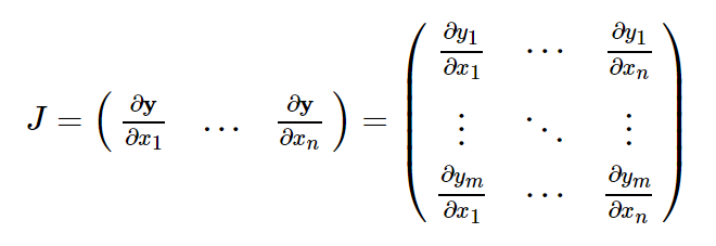
如果v恰好是标量函数的梯度，这里的标量也就是上面Q的gradient。

根据链式法则，vector-Jacobian ，external_grad表示v.

计算图

../../_img/dag_autograd.png

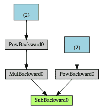
Autograd在右函数组成的有向无环图（DAG）中记录数据（张量）和所有已执行的操作（以及由此产生的新张量。），叶子数输入张量，根是输出张量。从根到叶子跟踪，使用链式法则自动计算梯度。

正向传播：

根据请求的操作计算结果
在DAG中维护操作对应参数的梯度函数

反向传播：

从每个.grad_fn计算梯度
累积保存在.grad属性中
根据链式法则，将梯度传播到叶子张量。

DAG图中，箭头是正向传播，节点代表相应的操作。蓝色节点就是叶张量a、b。

DAG在pytorch中是动态的，图是从头开始重新创建的，在每个.backward()调用之后，autograd开始填充新图，这也是允许在模型中使用控制流的原因，可以根据需要在每次迭代中改变形状、大小、操作。

从 DAG 中排除

import torch
#******************收集梯度******************#
x = torch.rand(5, 5)#不需要梯度的张量默认或者设置成requires_grad=False，会将其从梯度计算 DAG 中排除。
y = torch.rand(5, 5)
z = torch.rand((5, 5), requires_grad=True) # torch.autograd跟踪所有将其requires_grad标志设置为True的张量的操作
a = x + y
b = x + z # 即使只有一个输入张量具有requires_grad=True，操作的输出张量也将需要梯度。
print(f"Does `a` require gradients? : {a.requires_grad}")
print(f"Does `b` require gradients?: {b.requires_grad}")

在网络中，如果不需要计算梯度参数，就成为冻结参数，如微调迁移学习。

from torch import nn, optim
model = torchvision.models.resnet18(pretrained=True) # 加载一个预训练的 resnet18 模型
# Freeze all the parameters in the network
for param in model.parameters():
    param.requires_grad = False # 冻结所有参数
model.fc = nn.Linear(512, 10) # 分类器是最后一个线性层,换为分类器的新线性层（默认情况下未冻结）
 # 除了model.fc的参数外，模型中的所有参数都将冻结。 计算梯度的唯一参数是model.fc的权重和偏差
# Optimize only the classifier
optimizer = optim.SGD(model.fc.parameters(), lr=1e-2, momentum=0.9)#尽管我们在优化器中注册了所有参数，但唯一可计算梯度的参数（因此会在梯度下降中进行更新）是分类器的权重和偏差。
#torch.no_grad()中的上下文管理器可以使用相同的排除功能。

神经网络

nn依赖于autograd来定义模型并对其进行微分。nn.Module包含层，以及返回output的方法forward(input)。

convnet

import torch
import torch.nn as nn
import torch.nn.functional as F

class Net(nn.Module):
    def __init__(self):
        super(Net, self).__init__();
        # 1 input image channel, 6 output channels, 3x3 square convolution kernel
        self.conv1 = nn.Conv2d(1, 6, 3)
        self.conv2 = nn.Conv2d(6, 16, 3)
        # an affine operation: y = Wx + b
        self.fc1 = nn.Linear(16 * 6 * 6, 120) # 6*6 from image dimension
        self.fc2 = nn.Linear(120, 84)
        self.fc3 = nn.Linear(84, 10)
    def forward(self, x): # 只需要定义forward函数就可以使用autograd自动定义backward函数（计算梯度）
        # Max pooling over a (2, 2) window
        x = F.max_pool2d(F.relu(self.conv1(x)),(2,2)) # 32*32->30*30->15*15  ; conv: O=（I-K+2P）/S+1;
        # If the size is a square you can only specify a single number
        x = F.max_pool2d(F.relu(self.conv2(x)),2)#15*15->13*13->6*6
        x = x.view(-1, self.num_flat_features(x))#6*6
        x = F.relu(self.fc1(x))
        x = F.relu(self.fc2(x))
        x = self.fc3(x)
        return x
    def num_flat_features(self,x):
        size = x.size()[1:] # all dimensions except the batch dimension
        num_features = 1
        for s in size:
            num_features *= s
        return num_features
net = Net()
print(net)
params = list(net.parameters()) # 模型的可学习参数
print(len(params))
print(params[0].size()) # conv1's .weight
input = torch.randn(1, 1, 32, 32) # 输入大小为32，如何计算出来的呢
'''
Conv:
    输入图片（Input）大小为I*I，
    卷积核（Filter）大小为K*K，
    步长（stride）为S，
    填充（Padding）的像素数为P，那卷积层输出（Output）的特征图大小为O=（I-K+2P）/S+1
'''
out = net(input)
print(out)
net.zero_grad() # 反向传播梯度缓冲区归零
out.backward(torch.randn(1,10)) # 随机梯度作为参数梯度
#torch.nn 输入nSamples x nChannels x Height x Width的 4D 张量；只有一个样本，只需使用input.unsqueeze(0)添加一个假批量尺寸

torch.Tensor多维数组，支持backward()自动微分。
nn.Module神经网络模块。封装参数方便。
nn.Parameter张量，将其分配给module属性时，自动注册为参数
autograd.Function自动微分正向和反向定义，每一个tensor操作都会创建至少一个function节点，该节点连接到创建的tensor函数，并编码历史记录。

损失函数

import torch
import torch.nn as nn
import torch.nn.functional as F

class Net(nn.Module):
    def __init__(self):
        super(Net, self).__init__();
        # 1 input image channel, 6 output channels, 3x3 square convolution kernel
        self.conv1 = nn.Conv2d(1, 6, 3)
        self.conv2 = nn.Conv2d(6, 16, 3)
        # an affine operation: y = Wx + b
        self.fc1 = nn.Linear(16 * 6 * 6, 120) # 6*6 from image dimension
        self.fc2 = nn.Linear(120, 84)
        self.fc3 = nn.Linear(84, 10)
    def forward(self, x): # 只需要定义forward函数就可以使用autograd自动定义backward函数（计算梯度）
        # Max pooling over a (2, 2) window
        x = F.max_pool2d(F.relu(self.conv1(x)),(2,2)) # 32*32->30*30->15*15  ; conv: O=（I-K+2P）/S+1;
        # If the size is a square you can only specify a single number
        x = F.max_pool2d(F.relu(self.conv2(x)),2)#15*15->13*13->6*6
        x = x.view(-1, self.num_flat_features(x))#6*6
        x = F.relu(self.fc1(x))
        x = F.relu(self.fc2(x))
        x = self.fc3(x)
        return x
    def num_flat_features(self,x):
        size = x.size()[1:] # all dimensions except the batch dimension
        num_features = 1
        for s in size:
            num_features *= s
        return num_features
net = Net()
input = torch.randn(1, 1, 32, 32) # 输入大小为32，如何计算出来的呢
output = net(input)
target = torch.randn(10) # a dummy target, for example
target = target.view(1, -1) # make it the same shape as output
criterion = nn.MSELoss()
loss = criterion(output, target)
print(loss)
print(loss.grad_fn)  # MSELoss
print(loss.grad_fn.next_functions[0][0])  # Linear
print(loss.grad_fn.next_functions[0][0].next_functions[0][0])  # ReLU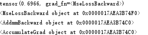

如果使用loss.grad_fn，就可以看到一个计算图

input -> conv2d -> relu -> maxpool2d -> conv2d -> relu -> maxpool2d
      -> view -> linear -> relu -> linear -> relu -> linear
      -> MSELoss
      -> loss

调用loss.backward()，整个图将被微分，且图中具有requires_grad=True的所有张量的.grad属性将会累积其张量。

反向传播

import torch
import torch.nn as nn
import torch.nn.functional as F

class Net(nn.Module):
    def __init__(self):
        super(Net, self).__init__();
        # 1 input image channel, 6 output channels, 3x3 square convolution kernel
        self.conv1 = nn.Conv2d(1, 6, 3)
        self.conv2 = nn.Conv2d(6, 16, 3)
        # an affine operation: y = Wx + b
        self.fc1 = nn.Linear(16 * 6 * 6, 120) # 6*6 from image dimension
        self.fc2 = nn.Linear(120, 84)
        self.fc3 = nn.Linear(84, 10)
    def forward(self, x): # 只需要定义forward函数就可以使用autograd自动定义backward函数（计算梯度）
        # Max pooling over a (2, 2) window
        x = F.max_pool2d(F.relu(self.conv1(x)),(2,2)) # 32*32->30*30->15*15  ; conv: O=（I-K+2P）/S+1;
        # If the size is a square you can only specify a single number
        x = F.max_pool2d(F.relu(self.conv2(x)),2)#15*15->13*13->6*6
        x = x.view(-1, self.num_flat_features(x))#6*6
        x = F.relu(self.fc1(x))
        x = F.relu(self.fc2(x))
        x = self.fc3(x)
        return x
    def num_flat_features(self,x):
        size = x.size()[1:] # all dimensions except the batch dimension
        num_features = 1
        for s in size:
            num_features *= s
        return num_features
net = Net()
input = torch.randn(1, 1, 32, 32) # 输入大小为32，如何计算出来的呢
output = net(input)
target = torch.randn(10) # a dummy target, for example
target = target.view(1, -1) # make it the same shape as output
criterion = nn.MSELoss()
loss = criterion(output, target)
net.zero_grad()     # zeroes the gradient buffers of all parameters 要清除现有的梯度，否则梯度将累积到现有的梯度中
print('conv1.bias.grad before backward')
print(net.conv1.bias.grad)
loss.backward()#反向传播
print('conv1.bias.grad after backward')
print(net.conv1.bias.grad)

更新权重

最简单的更新规则是随机梯度下降（SGD）：

weight = weight - learning_rate * gradient

learning_rate = 0.01
for f in net.parameters():
    f.data.sub_(f.grad.data * learning_rate)

import torch
import torch.nn as nn
import torch.nn.functional as F
import torch.optim as optim

class Net(nn.Module):
    def __init__(self):
        super(Net, self).__init__();
        # 1 input image channel, 6 output channels, 3x3 square convolution kernel
        self.conv1 = nn.Conv2d(1, 6, 3)
        self.conv2 = nn.Conv2d(6, 16, 3)
        # an affine operation: y = Wx + b
        self.fc1 = nn.Linear(16 * 6 * 6, 120) # 6*6 from image dimension
        self.fc2 = nn.Linear(120, 84)
        self.fc3 = nn.Linear(84, 10)
    def forward(self, x): # 只需要定义forward函数就可以使用autograd自动定义backward函数（计算梯度）
        # Max pooling over a (2, 2) window
        x = F.max_pool2d(F.relu(self.conv1(x)),(2,2)) # 32*32->30*30->15*15  ; conv: O=（I-K+2P）/S+1;
        # If the size is a square you can only specify a single number
        x = F.max_pool2d(F.relu(self.conv2(x)),2)#15*15->13*13->6*6
        x = x.view(-1, self.num_flat_features(x))#6*6
        x = F.relu(self.fc1(x))
        x = F.relu(self.fc2(x))
        x = self.fc3(x)
        return x
    def num_flat_features(self,x):
        size = x.size()[1:] # all dimensions except the batch dimension
        num_features = 1
        for s in size:
            num_features *= s
        return num_features
net = Net()
input = torch.randn(1, 1, 32, 32) # 输入大小为32，如何计算出来的呢
output = net(input)
target = torch.randn(10) # a dummy target, for example
target = target.view(1, -1) # make it the same shape as output

# create your optimizer
optimizer = optim.SGD(net.parameters(), lr=0.01)
# in your training loop:
optimizer.zero_grad()   # zero the gradient buffers将梯度缓冲区手动设置为零

criterion = nn.MSELoss()
loss = criterion(output, target)
loss.backward()#反向传播
optimizer.step()    # Does the update

训练分类器

数据

将数据加载到numpy然后转成torch.Tensor

图像，Pillow，OpenCV等
音频，SciPy和librosa
文本，基于python和Cython原始加载，NLTK和SpaCy

torchvision是针对视觉的包，包含常见数据集（Imagenet，CIFAR10，MNIST），以及用于数据加载工具（torchvision.datasets和torch.utils.data.DataLoader）。

CIFAR10 数据集。它具有以下类别：“飞机”，“汽车”，“鸟”，“猫”，“鹿”，“狗”，“青蛙”，“马”，“船”，“卡车”。 CIFAR-10 中的图像尺寸为3x32x32。

cifar10

训练图像分类器

使用torchvision加载并标准化CIFAR10数据集
定义网络模型
定义损失函数
训练
测试

import torch
import torchvision
import torchvision.transforms as transforms

import matplotlib.pyplot as plt
import numpy as np

import torch.nn as nn
import torch.nn.functional as F

import torch.optim as optim
def imshow(img):
    img = img / 2 +0.5 # unnormalize
    npimg = img.numpy()
    plt.imshow(np.transpose(npimg, (1, 2, 0)))
    plt.show()
# 加载并归一化图像
transform = transforms.Compose(
    [transforms.ToTensor(),
     transforms.Normalize((0.5, 0.5, 0.5), (0.5, 0.5, 0.5))])

trainset = torchvision.datasets.CIFAR10(root='./data', train=True, download=True, transform=transform)
trainloader = torch.utils.data.DataLoader(trainset, batch_size=4, shuffle=True, num_workers=0)

testset = torchvision.datasets.CIFAR10(root='./data', train=False, download=True, transform=transform)
testloader = torch.utils.data.DataLoader(testset, batch_size=4, shuffle=False, num_workers=0)

classes = ('plane', 'car', 'bird', 'cat', 'deer', 'dog', 'frog', 'horse', 'ship', 'truck')

# get some random training images
dataiter = iter(trainloader)
images, labels = dataiter.next()

#show images
imshow(torchvision.utils.make_grid(images))
# print labels
print(' '.join('%5s' % classes[labels[j]] for j in range(4)))
# 定义网络模型
class Net(nn.Module):
    def __init__(self):
        super(Net, self).__init__()
        self.conv1 = nn.Conv2d(3, 6, 5) # 三通道输入
        self.pool = nn.MaxPool2d(2, 2)
        self.conv2 = nn.Conv2d(6, 16, 5)
        self.fc1 = nn.Linear(16 * 5 * 5, 120)
        self.fc2 = nn.Linear(120, 84)
        self.fc3 = nn.Linear(84, 10)

    def forward(self, x):
        x = self.pool(F.relu(self.conv1(x)))
        x = self.pool(F.relu(self.conv2(x)))
        x = x.view(-1, 16 * 5 * 5)
        x = F.relu(self.fc1(x))
        x = F.relu(self.fc2(x))
        x = self.fc3(x)
        return x

net = Net()
# GPU训练
print(torch.cuda.is_available())
device = torch.device("cuda:0" if torch.cuda.is_available() else 'cpu')
# Assuming that we are on a CUDA machine, this should print a CUDA device:
print(device)
net.to(device)

# 定义损失函数
criterion = nn.CrossEntropyLoss()
# 定义优化器
optimizer = optim.SGD(net.parameters(), lr=0.001, momentum=0.9)
# 训练
for epoch in range(2): # loop over the dataset multiple times
    running_loss = 0.0
    for i, data in enumerate(trainloader, 0):
        # get the inputs; data is a list of [inputs, labels]
        # inputs, labels = data
        inputs, labels = data[0].to(device), data[1].to(device)

        # zero the parameter gradients
        optimizer.zero_grad()
        # forward
        outputs = net(inputs)
        loss = criterion(outputs, labels)
        # backward
        loss.backward()
        # optimize
        optimizer.step()

        # print statistics
        running_loss += loss.item()
        if i % 2000 == 1999: # print every 2000 mini-batches
            print('[%d, %5d] loss: %.3f'% (epoch + 1, i+1, running_loss / 2000))
            running_loss = 0.0
print('Finished Training')
# 保存模型
PATH = './cifar_net.pth'
torch.save(net.state_dict(), PATH)
# 测试
dataiter = iter(testloader)
images, labels = dataiter.next()

# print images
imshow(torchvision.utils.make_grid(images))
print('GroundTruth:  ',' '.join('%5s' % classes[labels[j]] for j in range(4)))

# 加载模型
net = Net()
net.to(device)
net.load_state_dict(torch.load(PATH))
# 预测
images = images.to(device)
outputs = net(images)
# 获取类别最大的概率
_, predicted = torch.max(outputs, 1)
print('Predicted: ', ' '.join('%5s' % classes[predicted[j]] for j in range(4)))
# 评价
correct = 0
total = 0
with torch.no_grad():
    for data in testloader:
        # images, labels = data
        images, labels = data[0].to(device), data[1].to(device)
        outputs = net(images)
        _, predicted = torch.max(outputs.data, 1)
        total += labels.size(0)
        correct += (predicted == labels).sum().item()
print('Accuracy of the network on the 10000 test images: %d %%' % (100 * correct /total))
class_correct = list(0. for i in range(10))
class_total = list(0. for i in range(10))
with torch.no_grad():
    for data in testloader:
        # images, labels = data
        images, labels = data[0].to(device), data[1].to(device)
        outputs = net(images)
        _, predicted = torch.max(outputs, 1)
        c = (predicted == labels).squeeze()
        for i in range(4):
            label = labels[i]
            class_correct[label] += c[i].item()
            class_total[label] += 1

for i in range(10):
    print('Accuracy of %5s: %2d %%'% (classes[i], 100 * class_correct[i] / class_total[i]))

shchojj

关注

0
点赞
踩
1

收藏

觉得还不错? 一键收藏
0
评论
PyTorch 深度学习（一）

https://pytorch.apachecn.org/docs/1.7/02.html最近没有正经看过源码，在回溯一下，以免忘记。pytorch有自动微分机制。张量可以理解为多维数组张量初始化import torchimport numpy as np#****************直接生成张量****************#data = [[1,2],[3,4]]x_data = torch.tensor(data)#***************numpy生成
复制链接

扫一扫