


https://www.nvidia.com/object/real-time-normal-map-dxt-compression.html
https://www.cnblogs.com/oiramario/archive/2011/03/18/1988351.html
Real-Time Normal Map DXT Compression
J.M.P. van Waveren | Ignacio Castaño |
February 7th 2008
© 2008, id Software, Inc.
Abstract
| Using today's graphics hardware, normal maps can be stored in several compressed formats, that are decompressed on the fly in hardware during rendering. Several object-space and tangent-space normal map compression techniques using existing texture compression formats are evaluated. While decompression from these formats happens in real-time in hardware during rendering, compression to these formats may take a considerable amount of time using existing compressors. Two highly optimized tangent-space normal map compression algorithms are presented that can be used to achieve real-time performance on both the CPU and GPU. |
1. Introduction
Bump mapping uses a texture to perturb the surface normal to give objects a more geometrically complex appearance without increasing the number of geometric primitives. Bump mapping, as originally described by Blinn [1], uses the gradient of a bump map heightfield to perturb the interpolated surface normal in the direction of the surface derivatives (tangent vectors), before calculating the illumination of the surface. By changing the surface normal, the surface is lit as if it has more detail, and as a result is also perceived to have more detail than the geometric primitives used to describe the surface.
Normal mapping is an application of bump mapping, and was introduced by Peercy et al. [2]. While bump mapping perturbs the existing surface normals of an object, normal mapping replaces the normals entirely. A normal map is a texture that stores normals. These normals are usually stored as unit-length vectors with three components: X, Y and Z. Normal mapping has significant performance benefits over bump mapping, in that far fewer operations are required to calculate the surface lighting.
Normal mapping is usually found in two varieties: object-space and tangent-space normal mapping. They differ in coordinate systems in which the normals are measured and stored. Object-space normal maps store normals relative to the position and orientation of a whole object. Tangent-space normals are stored relative to the interpolated tangent-space of the triangle vertices. While object-space normals can be anywhere on the unit-sphere, tangent-space normals are only on the unit-hemisphere at the front of the surface, because the normals always point out of the surface.
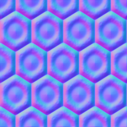
 |  |
| Example of an object-space normal map (left), and the same normal map in tangent-space (right). | |
A normal does not necessarily have to be stored as a vector with the components X, Y and Z. However, rendering from other representations usually comes at a performance cost. A normal could, for instance, be stored as an angle pair (pitch, yaw). However, this representation has the problem that interpolation or filtering does not work properly, because there are orientations in which there may not exist a simple change to the angles to represent a local rotation. Before interpolating, filtering, or calculating the surface illumination for that matter, the angle pair has to be converted to a different representation like a vector, which requires expensive trigonometric functions.
Although a normal map can be stored as a floating-point texture, a normal map is typically stored as a signed or unsigned integer texture, because the components of normal vectors take values within a well defined range (usually [-1, +1]), and there is a benefit to having the same precision across the whole range without wasting any bits for a floating-point exponent. For instance, to store a normal map as an unsigned integer texture with 8 bits per component, the X, Y and Z components are rescaled from real values in the range [-1, +1] to integer values in the range [0, 255]. As such, the real-valued vector [0, 0, 1] is converted to the integer vector [128, 128, 255], which, when interpreted as a point in RGB space, is the purple/blue color that is predominant in tangent-space normal maps. To render a normal map stored as an unsigned integer texture, the vector components are first mapped from an integer value to the floating-point range [0, +1] in hardware. For instance, in the case of a texture with 8 bits per component, the integer range [0, 255] is mapped to the floating-point range [0, +1] by division with 255. Then the components are typically mapped from the [0, +1] range to the [-1, +1] range during rendering in a fragment program by subtracting 1 after multiplication with 2. When a signed integer texture is used, the mapping from an integer value to the floating-point range [-1, +1] is performed directly in hardware.
Whether using a signed or unsigned integer texture, a fundamental problem is that it is not possible to derive a linear mapping from binary integer numbers to the floating-point range [-1, +1], such that the values -1, 0, and +1 are represented exactly. The mapping in hardware of signed integer textures, used in earlier NVIDIA implementations, does not exactly represent +1. For an n-bit unsigned integer component, the integer 0 maps to -1, the integer 2n-1 maps to 0, and the maximum integer value 2n-1 maps to 1 - 21-n. In other words, the values -1 and 0 are represented exactly, but the value +1 is not. The mapping used for DirectX 10 class hardware is non-linear. For an n-bit signed integer component, the integer -2n-1 maps to -1, the integer -2n-1+1 also maps to -1, the integer 0 maps to 0, and the integer 2n-1-1 maps to +1. In other words, the values -1, 0 and +1 are all represented exactly, but the value -1 is represented twice.
Signed textures are not supported on older hardware. Furthermore, the mapping from binary integers to the range [-1, +1] may be hardware specific. Some implementations may choose to not represent +1 exactly, whereas the conventional OpenGL mapping specifies that -1 and +1 can be represented exactly, but 0 can not. Other implementations may choose a non-linear mapping, or allow values outside the range [-1, +1], such that all three values -1, 0 and +1 can be represented exactly. To cover the widest range of hardware without any hardware specific dependencies, all normal maps used here are assumed to be stored as unsigned integer textures. The mapping from the range [0, +1] to [-1, +1] is performed in a fragment program by subtracting 1 after multiplication with 2. This may result in an additional fragment program instruction, which can be trivially removed when a signed texture is used. The mapping used here is the same as the conventional OpenGL mapping which results in an exact representation of the values -1 and +1, but not 0.
An integer normal map texture can typically be stored with 16 (5:6:5), 24 (8:8:8), 48 (16:16:16) or 96 (32:32:32) bits per normal vector. Most of today's normal maps, however, are stored with no more than 24 (8:8:8) bits per normal vector. It is important to realize there are relatively few 8:8:8 bit vectors that are actually close to unit-length. For instance, the integer vector [0, 0, 64], which is dark blue in RGB space, does not represent a unit-length normal vector (the length is 0.5 as opposed to 1.0). The following figure shows the percentage of representable 8:8:8 bit vectors that are less than a certain percentage off from being unit-length.

For instance, if it is not considered acceptable for normal vectors to be more than 5% from unit-length, then only about 15% of all representable 8:8:8 bit vectors can be used to represent normal vectors. Going to fewer bits of precision, like 5:6:5 bits, the number of representable vectors that are close to unit-length decreases quickly.
To significantly increase the number of vectors that can be used, each normal vector can be stored as a direction that is not necessarily unit-length. This direction then needs to be normalized in a fragment program. However, there is still some waste because only 83% of the all 8:8:8 bit vectors represent unique directions. For instance, the integer vectors [0, 0, 32], [0, 0, 64] and [0, 0, 96] all specify the exact same direction (they are multiples of each other). Furthermore, the unique normalized directions are not uniformly distributed over the unit-sphere. There are more representations for directions close to the four diagonals of the bounding box of the [-1, +1] x [-1, +1] x [-1, +1] vector space, than there are representations for directions close to the coordinate axes. For instance, there are three times more directions represented within a 15 degrees radius around the vector [1, 1, 1], than there are directions represented within a 15 degrees radius around the vector [0, 0, 1]. The figure below shows the distribution of all representable 8:8:8 bit vectors projected onto the unit-sphere. The areas with a low density of vectors are green, and the areas with a high density are red.
 |
| distribution of 8:8:8 bit vectors projected on the unit-sphere |
On today's graphics hardware, normal maps can also be stored in several compressed formats, that are decompressed in real-time during rendering. Compressed normal maps do not only require significantly less memory on the graphics card, but also generally render faster than uncompressed normal maps, due to reduced bandwidth requirements. Various different ways to exploit existing texture compression formats for normal map compression, have been suggested in literature [7, 8, 9]. Several of these normal map compression techniques, and extensions to them, are evaluated in section 2 and 3.
While decompression from these formats is done real-time in hardware, compression to these formats may take a considerable amount of time. Existing compressors are designed for high-quality off-line compression, not real-time compression [20, 21, 22]. However, real-time compression is quite useful for transcoding normal maps from a different format, compression of dynamically generated normal maps, and for compressed normal map render targets. In sections 4 and 5 two highly optimized tangent-space normal map compression algorithms are presented, that can be used to achieve real-time performance on both the CPU and GPU.
2. Object-Space Normal Maps
Object-space normal maps store normals relative to the position and orientation of a whole object. A normal in object-space can be anywhere on the full unit-sphere, and is typically stored as a vector with three components: X, Y and Z. Object-space normal maps can be stored using regular color texture compression techniques, but these techniques may not be as effective, because normal map textures do not have the same properties as color textures.
2.1 Object-Space DXT1
DXT1 [3, 4], also known as BC1 in DirectX 10 [5], is a lossy compression format for color textures, with a fixed compression ratio of 8:1. The DXT1 format is designed for real-time decompression in hardware on the graphics card during rendering. DXT1 compression is a form of Block Truncation Coding (BTC) [6] where an image is divided into non-overlapping blocks, and the pixels in each block are quantized to a limited number of values. The color values of pixels in a 4x4 pixel block are approximated with equidistant points on a line through RGB color space. This line is defined by two end-points, and for each pixel in the 4x4 block a 2-bit index is stored to one of the equidistant points on the line. The end-points of the line through color space are quantized to 16-bit 5:6:5 RGB format and either one or two intermediate points are generated through interpolation. The DXT1 format allows a 1-bit alpha channel to be encoded, by switching to a different mode based on the order of the end points, where only one intermediate point is generated and one additional color is specified, which is black and fully transparent.
Although the DXT1 format is designed for color textures this format can also be used to store normal maps. To compress a normal map to DXT1 format, the X, Y and Z components of the normal vectors are mapped to the RGB channels of a color texture. In particular for DXT1 compression each normal vector component is mapped from the range [-1, +1] to the integer range [0, 255]. The DXT1 format is decompressed in hardware during rasterization, and the integer range [0, 255] is mapped to the floating point range [0, 1] in hardware. In a fragment program the range [0, 1] will have to be mapped back to the range [-1, +1] to perform lighting calculations with the normal vectors. The following fragment program shows how this conversion can be implemented using a single instruction.
# input.x = normal.x  [0, 1]
# input.y = normal.y  [0, 1]
# input.z = normal.z  [0, 1]
# input.w = 0

MAD normal, input, 2.0, -1.0
Compressing a normal map to DXT1 format generally results in rather poor quality. There are noticeable blocking and banding artifacts. Only four distinct normal vectors can be encoded per 4x4 block, which is typically not enough to accurately represent all original normal vectors in a block. Because the normals in each block are approximated with equidistance points on a line, it is also impossible to encode four distinct normal vectors per 4x4 block that are all unit-length. Only two normal vectors per 4x4 block can be close to unit-length at a time, and usually a compressor selects a line through vector space which minimizes some error metric, such that, none of the vectors are actually close to unit-length.
 |  |
| The DXT1 compressed normal map on the right shows noticeable blocking artifacts compared to the original normal map on the left. | |
To improve the quality, each normal vector can be encoded as a direction that is not necessarily unit-length. This direction then has to be re-normalized in a fragment program. The following fragment program shows how a normal vector can be re-normalized.
# input.x = normal.x  [0, 1]
# input.y = normal.y  [0, 1]
# input.z = normal.z  [0, 1]
# input.w = 0

MAD normal, input, 2.0, -1.0
DP3 scale, normal, normal
RSQ scale.x, scale.x
MUL normal, normal, scale.x
Encoding directions gives the compressor more freedom, because the compressor does not have to worry about the magnitude of the vectors, and a much larger percentage of all representable vectors can be used for the end points of the line through normal space. However, this increased freedom makes compression a much harder problem.
|  |
| The DXT1 compressed normal map with re-normalization on the right compared to the original normal map on the left. | |
The above images show that, although the quality is a little bit better, the quality is generally still rather poor. Whether re-normalizing in a fragment program or not, the quality of DXT1 compressed object-space normal maps is generally not considered to be acceptable.
2.2 Object-Space DXT5
The DXT5 format [3, 4], also known as BC3 in DirectX 10 [5], stores three color channels the same way DXT1 does, but without 1-bit alpha channel. Instead of the 1-bit alpha channel, the DXT5 format stores a separate alpha channel which is compressed similarly to the DXT1 color channels. The alpha values in a 4x4 block are approximated with equidistant points on a line through alpha space. The end-points of the line through alpha space are stored as 8-bit values, and based on the order of the end-points either 4 or 6 intermediate points are generated through interpolation. For the case with 4 intermediate points, two additional points are generated, one for fully opaque and one for fully transparent. For each pixel in a 4x4 block a 3-bit index is stored to one of the equidistant points on the line through alpha space, or one of the two additional points for fully opaque or fully transparent. The same number of bits are used to encode the alpha channel as the three DXT1 color channels. As such, the alpha channel is stored with higher precision than each of the color channels, because the alpha space is one-dimensional, as opposed to the three-dimensional color space. Furthermore, there are a total of 8 samples to represent the alpha values in a 4x4 block, as opposed to 4 samples to represent the color values. Because of the additional alpha channel, the DXT5 format consumes twice the amount of memory of the DXT1 format.
The DXT5 format is designed for color textures with a smooth alpha channel. However, this format can also be used to store object-space normal maps. In particular, better quality normal map compression can be achieved by using the DXT5 format and moving one of the components to the alpha channel. By moving one of the components to the alpha channel this component is stored with more precision. Furthermore, by encoding only two components in the DXT1 block of the DXT5 format, the accuracy with which these components are stored typically improves as well. For object-space normal maps there is no clear benefit to moving any particular component to the alpha channel, because the normal vectors may point in any direction, and all values can occur with similar frequencies for all components. When an object-space normal map does have most vectors in a specific direction, then there is clearly a benefit to mapping the axis most orthogonal to that direction to the alpha channel. However, in general it is not practical to change the encoding on a per normal map basis, because a different fragment program is required for each encoding. The following fragment program assumes the Z component is moved to the alpha channel. The fragment program shows how the components are mapped from the range [0, 1] to the range [-1, +1], while the Z component is also moved back in place from the alpha channel.
# input.x = normal.x  [0, 1]
# input.y = normal.y  [0, 1]
# input.z = 0
# input.w = normal.z  [0, 1]

MAD normal, input.xywz, 2.0, -1.0
Just like DXT1 without re-normalization, this format results in minimal overhead in a fragment programs. The quality is significantly better than DXT1 compression of object-space normal maps. However, there are still noticeable blocking and banding artifacts.
|  |
| The DXT5 compressed normal map on the right compared to the original normal map on the left. | |
Using the third channel to store a scale factor like done for the YCoCg-DXT5 compression from [24] does not help much to improve the quality. The dynamic range of the individual components is typically too large, or the different components span different ranges that are far apart, while there is only one scale factor for the combined dynamic range.
Just like DXT1 compression of object-space normal maps, the quality can be improved by encoding a normal vector as a direction that is not necessarily unit-length. The following fragment program shows how to perform the swizzle and re-normalization.
# input.x = normal.x  [0, 1]
# input.y = normal.y  [0, 1]
# input.z = 0
# input.w = normal.z  [0, 1]

MAD normal, input.xywz, 2.0, -1.0
DP3 scale, normal, normal
RSQ scale.x, scale.x
MUL normal, normal, scale.x
Encoding directions gives the compressor a lot more freedom, because the compressor can ignore the magnitude of the vectors, and a much larger percentage of all representable vectors can be used for the end points of the lines through normal space. The normal vectors are encoded using both the DXT1 block of the DXT5 format and the alpha channel, where the end points of the alpha channel are stored without quantization. As such, the potential search space for the end points of the lines can be very large, and high quality compression may take a considerable amount of time.
|  |
| The DXT5 compressed normal map with re-normalization on the right compared to the original normal map on the left. | |
On current hardware, the DXT5 format with re-normalization in a fragment program results in the best quality compression of object-space normal maps.
3. Tangent-Space Normal Maps
Tangent-space normal vectors are stored relative to the interpolated tangent-space of the triangle vertices. Compression of tangent-space normal maps generally works better than compression of object-space normal maps, because the dynamic range is lower. The vectors are only on the unit-hemisphere at the front of the surface (the normal vectors never point into the object). Furthermore, most normal vectors are close to the tip of the unit-hemisphere with Z close to 1.
Using tangent-space normal maps in itself can be considered a form of compression compared to using object-space normal maps. A local transform is used to change the frequency domain of the vector components which reduces their storage requirements. The transform does require tangent vectors to be stored at the triangle vertices and, as such, comes at a cost. However, the storage requirements for the tangent vectors is relatively very small compared to the storage requirements for normal maps.
The compression of tangent-space normal maps can be improved by only storing the X and Y components of unit-length normal vectors, and deriving the Z components. The normal vectors are always pointing up out of the surface and the Z is always positive. Furthermore, the normal vectors are unit-length and, as such, the Z can be derived as follows.
Z = sqrt( 1 - X * X - Y * Y )
The problem with reconstructing Z from X and Y is that it is a non-linear operation, and breaks down under bilinear filtering. The problem is most noticeable when interpolating between two normals in the XY-plane. Ideally a normal map is scaled up using spherical interpolation of the normal vectors, where the interpolated samples follow the shortest great arc on the unit sphere at a constant speed. Bilinear filtering of a three component normal map, with re-normalization in the fragment program, does not result in spherical interpolation at a constant speed, but at least the interpolated samples follow the shortest great arc. With a two-component normal map, however, where the Z is derived from the X and Y, the interpolated samples no longer necessarily follow the shortest great arc on the unit sphere. For instance, interpolation between the two vectors in the figure below is expected to follow the dotted line. Instead, however, the interpolated samples are on the arc that goes up on the unit sphere.

Fortunately, real-world normal maps usually do not have many sharp normal boundaries with adjacent vectors close to the XY-plane, and most of the normals point straight up. As such, there are usually no noticeable artifacts when bilinearly or trilinearly filtering a two component normal map before deriving the Z components.
Only storing the X and Y components is in essence an orthographic projection of the normal vectors along the Z-axis onto the XY-plane. To reconstruct an original normal vector, a projection back onto the unit-hemisphere is used, by deriving the Z component from the X and Y. Instead of this orthographic projection, a stereographic projection can be used as well. For the stereographic projection the X and Y components are divided by one plus Z as follows, where (pX, pY) is the projection of the normal vector.
pX = X / ( 1 + Z )
pY = Y / ( 1 + Z )
The original normal vector is reconstructed by projecting the stereographically projected vector back onto the unit-hemisphere as follows.
denom = 2 / ( 1 + pX * pX + pY * pY )
X = pX * denom
Y = pY * denom
Z = denom - 1
The advantage of using the stereographic projection is that the interpolated normal vectors behave better under bilinear or trilinear filtering. The interpolated normal vectors are still not on the shortest great arc, but they are closer, and have less of a tendency to go up on the unit-hemisphere.
The stereographic projection also causes a more even distribution of the pX and pY components with the angle on the unit-hemisphere. Although this may seem desirable, it is actually not, because most tangent-space normal vectors are close to the tip of the unit-hemisphere. As such, there is actually an advantage to using the orthographic projection which results in more representations of vectors with Z close to 1. The compression techniques discussed below use the orthographic projection because for most normal maps it results in better quality compression.
3.1 Tangent-Space DXT1
Using tangent-space normal maps only the X and Y components have to be stored in the DXT1 format, and the Z component can be derived in a fragment program. The following fragment program shows how the Z can be derived from the X and Y.
# input.x = normal.x  [0, 1]
# input.y = normal.y  [0, 1]
# input.z = 0
# input.w = 0

MAD normal, input, 2.0, -1.0
DP4_SAT normal.z, normal, normal;
MAD normal, normal, { 1, 1, -1, 0 }, { 0, 0, 1, 0 };
RSQ temp, normal.z;
MUL normal.z, temp;
The following images show a XY_ DXT1 compressed normal map on the right, next to the original normal map on the left. The DXT1 compressed normal map shows noticeable blocking and banding artifacts.
 |  |
| XY_ DXT1 compressed normal map on the right compared to the original normal map on the left. | |
Although at first it may seem this kind of compression should produce superior quality, better quality compression can generally be achieved by storing all three components and re-normalizing in a fragment program, just like for object-space normal maps. When only the X and Y components are stored in the DXT1 format, the reconstructed normal vectors are automatically normalized by deriving the Z component. When the X and Y components are distorted due to the DXT1 compression, where all points are placed on a straight line through XY-space, the error in the derived Z can be quite large.
The fragment program shown below for re-normalizing the DXT1 compressed normals, is the same as the one used for DXT1 compressed object-space normal maps with re-normalization.
# input.x = normal.x  [0, 1]
# input.y = normal.y  [0, 1]
# input.z = normal.z  [0, 1]
# input.w = 0

MAD normal, input, 2.0, -1.0
DP3 scale, normal, normal
RSQ scale.x, scale.x
MUL normal, normal, scale.x
The following images show a DXT1 compressed normal map with re-normalization on the right, next to the original normal map on the left.
| |
| DXT1 compressed normal map with re-normalization on the right compared to the original normal map on the left. | |
Either way, whether only storing two components in the DXT1 and deriving the Z, or storing all three components in the DXT1 format with re-normalization in the fragment program, the quality is rather poor.
3.2 Tangent-Space DXT5
Just like for object-space normal maps, all three components can be stored in the DXT5 format. The best results are usually achieved when storing _YZX data. In other words the X component is moved to the alpha channel. This technique is also known as RxGB compression, and was employed in the computer game DOOM III. By moving the X component to the alpha channel, the X and Y components are encoded separately. This improves the quality because the X and Y components are most independent with the largest dynamic range. The Z is always positive and typically close to 1 and, as such, storing the Z component with the Y component in the DXT1 part of the DXT5 format causes little distortion of the Y component. Storing all three components results in minimal overhead in a fragment program as shown below.
# input.x = 0
# input.y = normal.y  [0, 1]
# input.z = normal.z  [0, 1]
# input.w = normal.x  [0, 1]

MAD normal, input.wyzx, 2.0, -1.0
The following images show that, although the quality is better than DXT1 compression, there are still noticeable banding artifacts.
|  |
| DXT5 compressed normal map on the right compared to the original normal map on the left. | |
Just like for object-space normal maps the quality can be improved by storing directions that are not necessarily unit-length. The best quality is typically achieved by also moving the X component to the DXT5 alpha channel. The following fragment program shows how the directions are re-normalized after moving the X component back in place from the alpha channel.
# input.x = normal.x  [0, 1]
# input.y = normal.y  [0, 1]
# input.z = 0
# input.w = normal.z  [0, 1]

MAD normal, input.wyzx, 2.0, -1.0
DP3 scale, normal, normal
RSQ scale.x, scale.x
MUL normal, normal, scale.x
The following images show that encoding directions with re-normalization in a fragment program reduces the banding artifacts, but they are still quite noticeable.
|  |
| The DXT5 compressed normal map with re-normalization on the right compared to the original normal map on the left. | |
For most tangent-space normal maps better quality compression can be achieved by only storing the X and Y components in the DXT5 format and deriving the Z. This is also known as DXT5nm compression, and is most popular in today's computer games. The following fragment program shows how the Z is derived from the X and Y components.
# input.x = 0
# input.y = normal.y  [0, 1]
# input.z = 0
# input.w = normal.x  [0, 1]

MAD normal, input.wyzx, 2.0, -1.0
DP4_SAT normal.z, normal, normal;
MAD normal, normal, { 1, 1, -1, 0 }, { 0, 0, 1, 0 };
RSQ temp, normal.z;
MUL normal.z, temp;
The following images show that only storing the X and Y and deriving the Z, further reduces the banding artifacts.
|  |
| DXT5 compressed normal map storing only X and Y on the right compared to the original normal map on the left. | |
When using XY_ DXT1, _YZX DXT5 or _Y_X DXT5 compression for tangent-space normal maps, there is at least one spare channel that can be used to store a scale factor, which can be used to counter quantization errors similar to what the YCoCg-DXT5 compressor from [24] does. However, trying to upscale the components to counter quantization errors does not improve the quality much (typically a PSNR improvement of less than 0.1 dB). The components can only be scaled up when they have a low dynamic range. Although most normals point straight up, and the magnitude of most X-Y vectors is relatively small, the dynamic range of the X-Y components is actually still quite large. Even if all normals never deviate more than 45 degrees from straight up, then each X or Y component may still map to the range [-cos( 45° ), +cos( 45° )], where cos( 45° ) ≅ 0.707. In other words even with a deviation of less than 45 degrees from straight up, which is 50% of the angular range, each component may still cover more than 70% of the maximum dynamic range. On one hand, this is a good thing, because for the components of tangent-space normal vectors this means the largest part of the dynamic range covers the most frequently occurring values. On the other hand this means it is hard to upscale the components because of a relatively large dynamic range.
In the case of the _Y_X DXT5 compression of tangent-space normal maps there are two unused channels, and one of these channels can be used to also store a bias to center the dynamic range. This significantly increases the number of 4x4 blocks for which the values can be scaled up (such that typically more than 75% of all 4x4 blocks use a scale factor of at least 2). However, even using a bias to increase the number of scaled 4x4 blocks does not help much to improve the quality. The real problem is that the four sample points of the DXT1 block are simply not enough to accurately represent all the Y components of the normals in a 4x4 block. Introducing more sample points would significantly improve the quality but this is obviously not possible within the DXT5 format.
Instead of storing a bias and scale, one of the spare channels can also be used to store a rotation of the normal vectors in a 4x4 block about the Z-axis, as suggested in [11, 12]. Such a rotation can be used to find a much tighter bounding box of the X-Y vectors. In particular using _Y_X DXT5 compression such a rotation can be used to make sure that the axis with the largest dynamic range maps to the alpha channel, which, as such, is compressed with more precision. To be able to map the axis with the largest dynamic range to the alpha channel, a rotation of up to 180 degrees may be required. This rotation can be stored as a constant value over the whole 4x4 block in one of the 5-bit channels. Instead of storing the angle of rotation, the cosine of the angle can be stored, such that the cosine does not have to be calculated in a fragment program where the vectors need to be rotated back to their original positions. The sine for a rotation in the range [0, 180] degrees is always positive and can, as such, trivially be derived from the cosine in a fragment program as follows.
sine = sqrt( 1 - cosine * cosine )
The PSNR improvement from rotating the normals in a 4x4 block is significant and typically in the range 2 to 3 dB. Unfortunately adjacent 4x4 blocks may need vastly different rotations, and under bilinear or trilinear filtering noticeable artifacts may appear for filtered texel samples at borders between two 4x4 blocks with different rotations. The X, Y and rotation are filtered separately before the rotation is applied to the X and Y components. As such, a filtered rotation is applied to filtered X and Y components, which is not the same as filtering X and Y components that are first rotated back to their original position. In other words, unless the normal map is only point sampled, using a rotation is also not an option to improve the quality of DXT1 or DXT5 normal map compression.
Of course a denormalization value can still be stored in one of the spare channels as described in [8]. The denormalization value is used to scale down the normal vectors for lower mip levels, such that specular highlights fade with distance to alleviate aliasing artifacts.
3.3 Tangent-Space 3Dc
The 3Dc format [10] is specifically designed for tangent-space normal map compression and produces much better quality than DXT1 or DXT5 normal map compression. The 3Dc format stores only two channels and, as such, cannot be used for object-space normal maps. The format basically consists of two DXT5 alpha blocks for each 4x4 block of normals. In other words for each 4x4 block there are 8 samples for the X components and also 8 independent samples for the Y components. The Z components have to be derived in a fragment program.
The 3Dc format is also known as BC5 in DirectX 10 [5]. The same format can be loaded in OpenGL as LATC or RGTC. Using the LATC format the luminance is replicated in all three RGB channels. This can be particularly convenient, because this way the same swizzle (and fragment program code) can be used for both LATC and _Y_X DXT5 (DXT5nm) compressed normal maps. In other words the same fragment program can be used on hardware that does, and does not support 3Dc. The following fragment program shows how the Z is derived from the X and Y components when the normal map is stored in RGTC format.
# normal.x = x  [0, 1]
# normal.y = y  [0, 1]
# normal.z = 0
# normal.w = 0

MAD normal, normal, 2.0, -1.0
DP4 normal.z, normal, normal;
MAD normal, normal, { 1.0, 1.0, -1, 0 }, { 0, 0, 1, 0 };
RSQ temp, normal.z;
MUL normal.z, temp;
The following images show how 3Dc compression of normal maps, results in significantly less banding compared to _Y_X DXT5 (DXT5nm).
|  |
| 3Dc compressed normal map on the right compared to the original normal map on the left. | |
Several extensions to 3Dc are proposed in [11] and a new format specifically designed for improved normal map compression is presented in [12]. However, these formats are not available in current graphics hardware. On all DirectX 10 compatible hardware the 3Dc (or BC5) format results in the best quality tangent-space normal map compression. On older hardware which does not implement 3Dc the best quality is generally achieved using _Y_X DXT5 (DXT5nm).
4. Real-Time Compression on the CPU
While decompression from the formats described in the previous sections is done real-time in hardware, compression to these formats may take a considerable amount of time. Existing compressors are designed for high-quality off-line compression, not real-time compression [20, 21, 22]. However, real-time compression is quite useful to compress normal maps that are stored on disk in a different (more space efficient) format, and to compress dynamically generated normal maps.
In today's rendering engines, tangent-space normal maps are far more popular than object-space normal maps. On current hardware there are no compression formats available for object-space normal maps that work really well. The object-space normal map compression techniques described in section 2 all result in noticeable artifacts, or the compression is exceedingly expensive.
An object-space normal map can also not be used on an animated object. While the object surface animates the object-space normal vectors stay pointing in the same object-space direction. Tangent-space normal maps on the other hand, store normals relative to the tangent-space at the triangle vertices. When the surface of an object animates and the tangent vectors (stored at the triangle vertices) are transformed with the surface, the tangent-space normal vectors that are stored relative to these tangent vectors will also animate with the surface. As such the focus here is on real-time compression of tangent-space normal maps.
On hardware where the 3Dc (BC5 or LATC) format is not available, the _Y_X DXT5 (DXT5nm) format generally results in the best quality tangent-space normal map compression. The real-time _Y_X DXT5 compressor is very similar to the real-time DXT5 compressor from [23].
First the bounding box of X-Y normal space is calculated. The two lines that are used to approximate the X and Y-values go from the minimums to the maximums of this bounding box. To improve the Mean Square Error (MSE), the bounding box is inset on either end with a quarter the distance between the sample points on the lines. The Y components are stored in the "green" channel and there are 4 sample points on the line through "color" space. As such, the minimum and maximum Y values are inset with 1/16th of the range. The X components are stored in the "alpha" channel and there are 8 sample points on the line through "alpha" space. As such, the minimum and maximum X values are inset with 1/32nd of the range. The inset is implemented such that the minimum and maximum values are rounded outwards just like the YCoCg-DXT5 compressor from [24] does.
Only a single channel of the "color" channels is used to store the Y components of the normal vectors. Using this knowledge, the real-time DXT5 compressor from [23] can be optimized further specifically for _Y_X DXT5 compression. The best matching points on the line through Y-space can be found in a similar way the best matching points on the line through "alpha" space are found in the DXT5 compressor from [23]. First a set of cross-over points are calculated where a Y value goes from being closest to one sample point to another.
byte mid = ( max - min ) / ( 2 * 3 );

byte gb1 = max - mid;
byte gb2 = ( 2 * max + 1 * min ) / 3 - mid;
byte gb3 = ( 1 * max + 2 * min ) / 3 - mid;
A Y value can then be tested for being greater-equal to each of the cross-over points, and the results of these comparisons (0 for false and 1 for true) can be added together to calculate an index. This results in the following order where index 0 through 3 go from the minimum to the maximum.
|
However, the "color" sample points are ordered differently in the DXT5 format as follows.
|
Subtracting the results of the comparisons from four, and wrapping the result with a bitwise logical AND with 3, results in the following order.
|
The order is close to correct, but the min and max are still swapped. The following code shows how the Y values are compared to the cross-over points, and how the indices are calculated from the results of the comparisons, where index 0 and 1 are swapped at the end by XOR-ing with the result of the comparison ( 2 > index ).
unsigned int result = 0;
for ( int i = 15; i >= 0; i-- ) {
    result <<= 2;
    byte g = block[i*4];
    int b1 = ( g >= gb1 );
    int b2 = ( g >= gb2 );
    int b3 = ( g >= gb3 );
    int index = ( 4 - b1 - b2 - b3 ) & 3;
    index ^= ( 2 > index );
    result |= index;
}
Using SIMD instructions each byte comparison results in a byte with either all zero bits (when the expression is false), or all one bits (when the expression is true). When interpreted as a signed (two's-complements) integer, the result of a byte comparison is equal to either the number 0 (for false) or the number -1 (for true). Instead of explicitly subtracting a 1 for a comparison that results in true, the actual result of the comparison can simply be added to the value four as a signed integer.
The calculation of the indices for the "alpha" channel is very similar to the calculation used in the real-time DXT5 compressor from [23]. However, the calculation can be optimized further by also selecting the best matching sample points with subtraction as opposed to addition. First a set of cross-over points are calculated where an X value goes from being closest to one sample point to another.
byte mid = ( max - min ) / ( 2 * 7 );

byte ab1 = max - mid;
byte ab2 = ( 6 * max + 1 * min ) / 7 - mid;
byte ab3 = ( 5 * max + 2 * min ) / 7 - mid;
byte ab4 = ( 4 * max + 3 * min ) / 7 - mid;
byte ab5 = ( 3 * max + 4 * min ) / 7 - mid;
byte ab6 = ( 2 * max + 5 * min ) / 7 - mid;
byte ab7 = ( 1 * max + 6 * min ) / 7 - mid;
An X value can then be tested for being greater-equal to each of the cross-over points, and the results of these comparisons (0 for false and 1 for true) can be subtracted from 8 and wrapped using a bitwise logical AND with 7 to calculate the index. The first two indices are also swapped by xoring with the result of the comparison ( 2 > index ) as shown in the following code.
byte indices[16];
for ( int i = 0; i < 16; i++ ) {
    byte a = block[i*4];
    int b1 = ( a >= ab1 );
    int b2 = ( a >= ab2 );
    int b3 = ( a >= ab3 );
    int b4 = ( a >= ab4 );
    int b5 = ( a >= ab5 );
    int b6 = ( a >= ab6 );
    int b7 = ( a >= ab7 );
    int index = ( 8 - b1 - b2 - b3 - b4 - b5 - b6 - b7 ) & 7;
    indices[i] = index ^ ( 2 > index );
}
The full implementation of the real-time _Y_X DXT5 compressor can be found in appendix A. MMX and SSE2 implementations of this real-time compressor can be found in appendix B and C respectively.
Where available, the 3Dc (BC5 or LATC) format results in the best quality tangent-space normal map compression. The real-time 3Dc compressor first calculates the bounding box of X-Y normal space just like the _Y_X DXT5 compressor does. The two lines that are used to approximate the X and Y-values go from the minimums to the maximums of this bounding box. To improve the Mean Square Error (MSE), the bounding box is inset on either end with a quarter the distance between the sample points on the lines. The 3Dc format basically stores two DXT5 alpha channels both with the same encoding and 8 sample points. As such, on both axes the bounding box is inset on either end with 1/32th of the range. The same code as used for the _Y_X DXT5 compression, is used here as well to calculate the "alpha" channel indices, except that it is used twice. The full implementation of the real-time 3Dc compressor can be found in appendix A. MMX and SSE2 implementations of this real-time compressor can be found in appendix B and C respectively.
5. Real-Time Compression on the GPU
Real-time compression of tangent-space normal maps can also be performed on the GPU. This is possible thanks to new features available on DX10-class graphics hardware that enable rendering to integer textures and the use of bitwise and arithmetic integer operations..
To compress a normal map, a fragment program is used for each block of 4x4 texels by rendering a quad over the entire destination surface. The result of this fragment program is a compressed DXT block that is written to the texels of an integer texture. Both, DXT5 and 3Dc blocks are 128 bits, which is equal to one RGBA texel with 32 bits per component. As such, an unsigned integer RGBA texture is used as the render target when compressing a normal map to either format. The contents of this render target are then copied to the corresponding DXT texture by using Pixel Buffer Objects. This process is very similar to the one used for YCoCg-DXT5 compression that is described in more detail in [24].
3Dc compressed textures are exposed in OpenGL through two different extensions: GL_EXT_texture_compression_latc [25], and GL_EXT_texture_compression_rgtc [26]. The former maps the X and Y components to the luminance and alpha channels, while the latter maps the X and Y components to red and green respectively, where the remaining channels are set to 0.
In the implementation described here the LATC format is used. This is slightly more convenient, because it allows sharing the same shader code used for the normal reconstruction:
N.xy = 2 * tex2D(image, texcoord).wy - 1;
N.z = sqrt(saturate(1 - N.x * N.x - N.y * N.y));
When using LATC the luminance is replicated in the RGB channels, so the W-Y swizzle maps the luminance and alpha components to X and Y. Similarly, when using _Y_X DXT5, the W-Y swizzle maps the green and alpha components to X and Y.
The same code as used in [24] to encode the alpha channel for YCoCg-DXT5 compression, can also be used to encode the X and Y components for 3Dc compression, and the X component for _Y_X DXT5 compression. As shown in Section 4, the _Y_X DXT5 compressor can also be optimized to compute the DXT1 block by fitting only the Y component. However, as noted in [23], the alpha space is a one-dimensional space and the points on the line through alpha space are equidistant, which allows the closest point for each original alpha value to be calculated through division. On the CPU this requires a rather slow scalar integer division, because there are no MMX or SSE2 instructions available for integer division. The division can be implemented as an integer multiplication with a shift. However, the divisor is not a constant which means a lookup table is required to get the multiplier. Multiplication also increases the dynamic range which limits the amount of parallelism that can be exploited through a SIMD instruction set. On the CPU there is a clear benefit to exploiting maximum parallelism by using simple operations on the smallest possible elements (bytes) without increasing the dynamic range. However, on the GPU, scalar floating point math is used, and a division and/or multiplication is relatively cheap. As such, the X and Y components can be mapped to the respective indices by applying only a scale and a bias. The CG code for the index calculation of the Y component for the _Y_X DXT5 format is as follows:
const int GREEN_RANGE = 3;

float bias = maxGreen + (maxGreen - minGreen) / (2.0 * GREEN_RANGE);
float scale = 1.0f / (maxGreen - minGreen);

// Compute indices
uint indices = 0;
for (int i = 0; i < 16; i++)
{
    uint index = saturate((bias - block[i].y) * scale) * GREEN_RANGE;
    indices |= index << (i * 2);
}

uint i0 = (indices & 0x55555555);
uint i1 = (indices & 0xAAAAAAAA) >> 1;
indices = ((i0 ^ i1) << 1) | i1;
The same can be done for the X component of the _Y_X DXT5 format, and for both the X and Y component of the 3Dc format:
const int ALPHA_RANGE = 7;

float bias = maxAlpha + (maxAlpha - minAlpha) / (2.0 * ALPHA_RANGE);
float scale = 1.0f / (maxAlpha - minAlpha);

uint2 indices = 0;

for (int i = 0; i < 6; i++)
{
    uint index = saturate((bias - block[i].x) * scale) * ALPHA_RANGE;
    indices.x |= index << (3 * i);
}

for (int i = 6; i < 16; i++)
{
    uint index = saturate((bias - block[i].x) * scale) * ALPHA_RANGE;
    indices.y |= index << (3 * i - 18);
}

uint2 i0 = (indices >> 0) & 0x09249249;
uint2 i1 = (indices >> 1) & 0x09249249;
uint2 i2 = (indices >> 2) & 0x09249249;

i2 ^= i0 & i1;
i1 ^= i0;
i0 ^= (i1 | i2);

indices.x = (i2.x << 2) | (i1.x << 1) | i0.x;
indices.y = (((i2.y << 2) | (i1.y << 1) | i0.y) << 2) | (indices.x >> 16);
indices.x <<= 16;
The full Cg 2.0 implementations of the real-time _Y_X DXT5 (DXT5nm) normal map compressor, and the real-time 3Dc (BC5 or LATC) normal map compressor, can be found in appendix D.
6. Compression on the CPU vs. GPU
As shown in the previous sections high performance normal map compression can be implemented on both the CPU and the GPU. Whether the compression is best implemented on the CPU or the GPU is application dependent.
Real-time compression on the CPU is useful for normal maps that are dynamically created on the CPU. Compression on the CPU is also particularly useful for transcoding normal maps that are streamed from disk in a format that cannot be used for rendering. For example, a normal map or a height map may be stored in JPEG format on disk and, as such, cannot be used directly for rendering. Only some parts of the JPEG decompression algorithm can currently be implemented efficiently on the GPU. Memory can be saved on the graphics card, and rendering performance can be improved, by decompressing the original data and re-compressing it to DXT format. The advantage of re-compressing the texture data on the CPU is that the amount of data uploaded to the graphics card is minimal. Furthermore, when the compression is performed on the CPU, the full GPU can be used for rendering work as it does not need to perform any compression. With a definite trend to a growing number of cores on today's CPUs, there are typically free cores laying around that can easily be used for texture compression.
Real-time compression on the GPU may be less useful for transcoding, because of increased bandwidth requirements for uploading uncompressed texture data and because the GPU may already be tasked with expensive rendering work. However, real-time compression on the GPU is very useful for compressed render targets. The compression on the GPU can be used to save memory when rendering to a texture. Furthermore, such compressed render targets can improve the performance if the data from the render target is used for further rendering. The render target is compressed once, while the resulting data may be accessed many times during rendering. The compressed data results in reduced bandwidth requirements during rasterization and can, as such, significantly improve performance.
7. Results
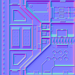
7.1 Object-Space
The object-space normal map compression techniques have been tested with the object-space normal maps shown below.
| Object-Space Normal Maps | |||
 |  |  | |
| 1. arcade | 2. tentacle | 3. chest | 4. face |
The Peak Signal to Noise Ratio (PSNR) has been calculated over the unweighted X, Y and Z values, stored as 8-bit unsigned integers.
| PSNR | ||||||||
| image | XYZ DXT1 | re-normalized XYZ DXT1 | XY_Z DXT5 | re-normalized XY_Z DXT5 | ||||
|---|---|---|---|---|---|---|---|---|
| 01_arcade | 30.90 | 32.95 | 34.02 | 37.23 | ||||
| 02_tentacle | 36.68 | 38.29 | 41.04 | 41.62 | ||||
| 03_chest | 39.24 | 40.79 | 42.22 | 43.47 | ||||
| 04_face | 37.38 | 38.99 | 41.03 | 42.60 | ||||

7.2 Tangent-Space
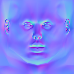
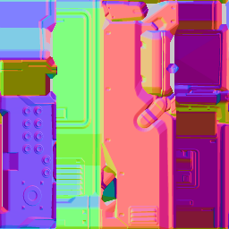
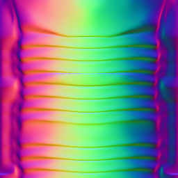
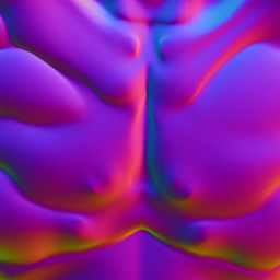
The tangent-space normal map compression techniques have been tested with the tangent-space normal maps shown below.
| Tangent-Space Normal Maps | |||
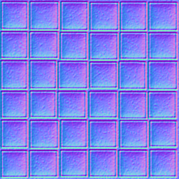 |  |  |  |
| 1. dot1 | 2. dot2 | 3. dot3 | 4. dot4 |
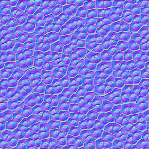
 |  |  |  |
| 5. lumpy | 6. voronoi | 7. turtle | 8. normalmap |
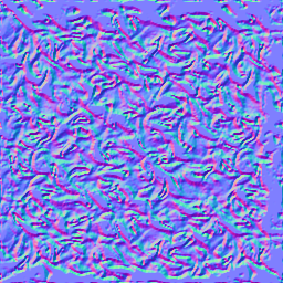
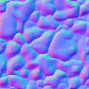
 | 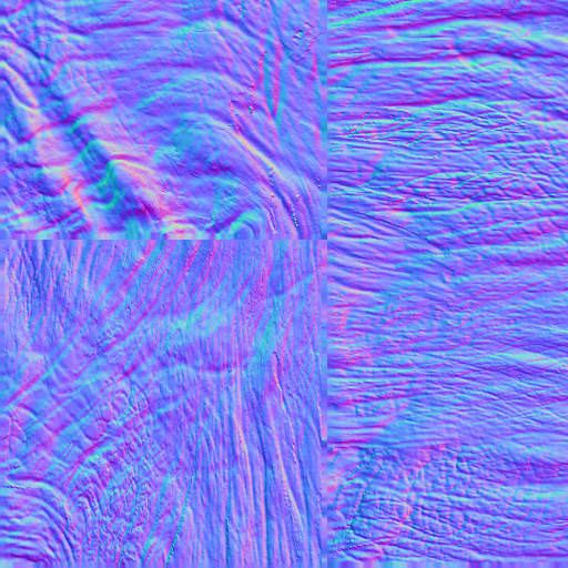 | 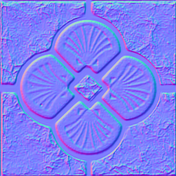 |  |
| 9. metal | 10. skin | 11. onetile | 12. barrel |
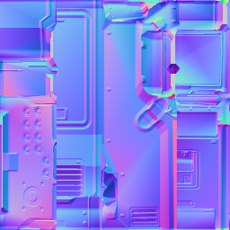 | 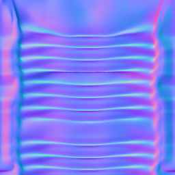 | 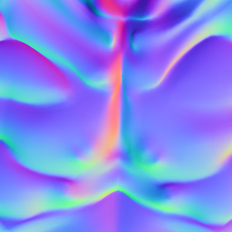 | |
| 13. arcade | 14. tentacle | 15. chest | 16. face |
The Peak Signal to Noise Ratio (PSNR) has been calculated over the unweighted X, Y and Z values, stored as 8-bit unsigned integers.
| PSNR | ||||||||||||
| image | XY_ DXT1 | re-normalized XYZ DXT1 | _YZX DXT5 | re-normalized _YZX DXT5 | _Y_X DXT5 | 3Dc | ||||||
|---|---|---|---|---|---|---|---|---|---|---|---|---|
| 01_dot1 | 27.61 | 29.51 | 32.00 | 35.16 | 35.07 | 40.15 | ||||||
| 02_dot2 | 25.39 | 26.45 | 29.55 | 32.92 | 32.68 | 36.70 | ||||||
| 03_dot3 | 21.88 | 23.05 | 27.34 | 30.77 | 30.02 | 34.13 | ||||||
| 04_dot4 | 23.18 | 24.46 | 29.16 | 32.81 | 31.38 | 35.80 | ||||||
| 05_lumpy | 30.54 | 31.13 | 34.70 | 37.15 | 37.73 | 41.92 | ||||||
| 06_voronoi | 37.53 | 38.16 | 41.72 | 42.16 | 43.93 | 48.23 | ||||||
| 07_turtle | 36.12 | 37.06 | 38.74 | 39.93 | 41.22 | 45.76 | ||||||
| 08_normalmap | 35.57 | 36.36 | 37.78 | 38.95 | 40.00 | 44.49 | ||||||
| 09_metal | 41.65 | 41.99 | 46.37 | 46.55 | 49.03 | 54.10 | ||||||
| 10_skin | 28.95 | 29.48 | 34.68 | 36.20 | 36.83 | 41.37 | ||||||
| 11_onetile | 29.08 | 29.82 | 34.17 | 35.98 | 36.76 | 41.14 | ||||||
| 12_barrel | 29.93 | 31.67 | 33.15 | 36.79 | 37.03 | 40.20 | ||||||
| 13_arcade | 32.31 | 33.63 | 36.86 | 39.24 | 39.81 | 44.61 | ||||||
| 14_tentacle | 39.03 | 40.47 | 40.30 | 41.39 | 43.23 | 47.82 | ||||||
| 15_chest | 38.92 | 41.03 | 41.64 | 42.29 | 42.87 | 46.52 | ||||||
| 16_face | 38.27 | 39.58 | 41.59 | 42.55 | 43.71 | 48.61 | ||||||

The following graph uses the 3Dc format to show the quality difference between the orthographic and stereographic projections. The stereographic projection results in more consistent results but for most normal maps the quality is significantly lower.

The following graph is only of theoretical interest, in that it shows the quality improvement from rotating the normals in a 4x4 block, and storing the rotation in one of the unused channels in the _Y_X DXT5 format. The graph shows the quality improvement for normal maps that are only point sampled, because filtering causes noticeable artifacts for texel samples between 4x4 blocks with different rotations.

7.3 Real-Time Tangent-Space
The real-time tangent-space normal map compressors have been tested with the same tangent-space normal maps shown above. The Peak Signal to Noise Ratio (PSNR) has been calculated over the unweighted X, Y and Z values, stored as 8-bit unsigned integers.
| PSNR | ||||||||
| image | off-line _Y_X DXT5 | real-time _Y_X DXT5 | off-line 3Dc | real-time 3Dc | ||||
|---|---|---|---|---|---|---|---|---|
| 01_dot1 | 35.07 | 33.36 | 40.15 | 37.99 | ||||
| 02_dot2 | 32.68 | 31.67 | 36.70 | 35.67 | ||||
| 03_dot3 | 30.02 | 29.03 | 34.13 | 33.22 | ||||
| 04_dot4 | 31.38 | 30.49 | 35.80 | 34.89 | ||||
| 05_lumpy | 37.73 | 36.63 | 41.92 | 40.63 | ||||
| 06_voronoi | 43.93 | 42.99 | 48.23 | 46.99 | ||||
| 07_turtle | 41.22 | 40.30 | 45.76 | 44.50 | ||||
| 08_normalmap | 40.00 | 38.99 | 44.49 | 43.26 | ||||
| 09_metal | 49.03 | 47.60 | 54.10 | 52.45 | ||||
| 10_skin | 36.83 | 35.69 | 41.37 | 40.20 | ||||
| 11_onetile | 36.76 | 35.67 | 41.14 | 39.92 | ||||
| 12_barrel | 37.03 | 35.51 | 40.20 | 39.11 | ||||
| 13_arcade | 39.81 | 38.05 | 44.61 | 42.18 | ||||
| 14_tentacle | 43.23 | 41.90 | 47.82 | 46.31 | ||||
| 15_chest | 42.87 | 41.95 | 46.52 | 45.38 | ||||
| 16_face | 43.71 | 42.85 | 48.61 | 47.53 | ||||

The performance of the SIMD optimized real-time compressors has been tested on an Intel® 2.8 GHz dual-core Xeon® ("Paxville" 90nm NetBurst microarchitecture) and an Intel® 2.9 GHz Core™2 Extreme ("Conroe" 65nm Core 2 microarchitecture). Only a single core of these processors was used for the compression. Since the texture compression is block based, the compression algorithms can easily use multiple threads to utilize all cores of these processors. When using multiple cores there is an expected linear speed up with the number of available cores. The performance of the Cg 2.0 implementations has also been tested on a NVIDIA GeForce 8600 GTS and a NVIDIA GeForce 8800 GTX.
The following figure shows the number of Mega Pixels that can be compressed to the _Y_X DXT5 format per second (higher MP/s = better).

The following figure shows the number of Mega Pixels that can be compressed to the 3Dc format per second (higher MP/s = better).

8. Conclusion
Existing color texture compression formats can also be used to store normal maps, but the results vary. The latest graphics hardware also implements formats specifically designed for normal map compression. While decompression from these formats happens in real-time in hardware during rendering, compression to these formats may take a considerable amount of time. Existing compressors are designed for high-quality off-line compression, not real-time compression. However, at the cost of a little quality, normal maps can also be compressed real-time on both the CPU and GPU, which is useful for transcoding normal maps from a different format and compression of dynamically generated normal maps.


 1万+
1万+

 被折叠的 条评论
为什么被折叠?
被折叠的 条评论
为什么被折叠?
 到【灌水乐园】发言


