Bundle Adjustment
在上一篇文章中,成功将三维重建扩展到了任意数量的图像,但是,随着图像的增多,累计误差会越来越大,从而影响最终的重建效果。要解决这个问题,需要用到Bundle Adjustment(下文简称BA)。
BA本质上是一个非线性优化算法,先来看看它的原型
minx∑iρi(||fi(xi1,xi2,...,xik)||2)
其中
x
是我们需要优化的参数,
f
一般称为代价函数(Cost Function),
ρ
为损失函数(Loss Function)。其中
f
的返回值可能是一个向量,因此总的代价取该向量的2-范数。
对于三维重建中的BA,代价函数往往是反向投影误差,比如我们需要优化的参数有相机的内参(焦距、光心、畸变等)、外参(旋转和平移)以及点云,设图像
i
的内参为
Ki
,外参为
Ri
和
Ti
,点云中某一点的坐标为
Pj
,该点在
i
图像中的像素坐标为
pij
,则可以写出反向投影误差
f(Ki,Ri,Ti,Pj)=π(Ki[Ri Ti]Pj)−pij
上式中的
Pj
和
pij
均为齐次坐标,其中
π
为投影函数,有
π(p)=(px/pz, py/pz, 1)
.
而损失函数
ρ
的目的是为了增强算法的鲁棒性,使得算法不易受离群点(Outliers)的影响,常见的有Huber函数、Tukey函数等,这些函数的图像如下
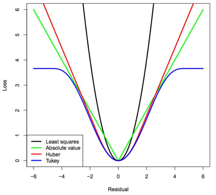
若不使用损失函数,即
ρ(x)=x
,那么就如上图中的黑色曲线,代价(Cost)随着误差以二次幂的速度增长,也许一个误差较大的点,就能左右算法的优化方向。其他的损失函数,可以发现,随着误差的增大,要么代价的增长是趋于线性的(Huber),要么干脆趋于不变(Tukey),这样就降低了误差较大的点对总代价的影响。损失函数实际上就是代价的重映射过程。
Ceres Solver
如何求解BA?总体思想是使用梯度下降,比如高斯-牛顿迭代、Levenberg-Marquardt算法等,由于BA还有自己的一些特殊性,比如稀疏性,在实现时还有很多细节需要处理,在此就不细说了。好在现在有很多用于求解非线性最小二次问题的库,文中使用的就是Google的一个开源项目——Ceres Solver.
Ceres Solver专为求解此类问题进行了大量的优化,有很高的效率,尤其在大规模问题上,其优势更加明显。并且,Ceres内置了一些常用的函数,比如对坐标的旋转以及各类损失函数,使其在开发上也比较高效。在官网上可以找到它的编译方法和使用教程,Windows用户可以在此找到配置好的VS工程。
编写代码
代码总体基本不变,我们只需要再添加一个函数用于BA即可,还有一点需要注意的是,Ceres Solver默认使用双精度浮点,如果精度不够可能导致计算梯度失败、问题无法收敛等问题,因此在原来的代码中,需要将原本问Point3f型的structure,改为Point3d类型。
首先定义一个代价函数
struct ReprojectCost
{
cv::Point2d observation;
ReprojectCost(cv::Point2d& observation)
: observation(observation)
{
}
template <typename T>
bool operator()(const T* const intrinsic, const T* const extrinsic, const T* const pos3d, T* residuals) const
{
const T* r = extrinsic;
const T* t = &extrinsic[3];
T pos_proj[3];
ceres::AngleAxisRotatePoint(r, pos3d, pos_proj);
pos_proj[0] += t[0];
pos_proj[1] += t[1];
pos_proj[2] += t[2];
const T x = pos_proj[0] / pos_proj[2];
const T y = pos_proj[1] / pos_proj[2];
const T fx = intrinsic[0];
const T fy = intrinsic[1];
const T cx = intrinsic[2];
const T cy = intrinsic[3];
const T u = fx * x + cx;
const T v = fy * y + cy;
residuals[0] = u - T(observation.x);
residuals[1] = v - T(observation.y);
return true;
}
};
- 1
- 2
- 3
- 4
- 5
- 6
- 7
- 8
- 9
- 10
- 11
- 12
- 13
- 14
- 15
- 16
- 17
- 18
- 19
- 20
- 21
- 22
- 23
- 24
- 25
- 26
- 27
- 28
- 29
- 30
- 31
- 32
- 33
- 34
- 35
- 36
- 37
- 38
- 39
- 40
- 41
该代价函数就是之前所说的反向投影误差,参数分别为内参、外参还有点在空间中的坐标,最后一个参数用于输出,为反向投影误差。注意,为了使BA更高效可靠,外参当中的旋转部分使用的是旋转向量而不是旋转矩阵,这样不仅使优化参数从9个变为3个,还能保证参数始终代表一个合法的旋转(如果用矩阵,可能在优化过程中,正交性不再满足)。
接下来直接使用Ceres Solver求解BA,其中使用了Ceres提供的Huber函数作为损失函数
void bundle_adjustment(
Mat& intrinsic,
vector<Mat>& extrinsics,
vector<vector<int>>& correspond_struct_idx,
vector<vector<KeyPoint>>& key_points_for_all,
vector<Point3d>& structure
)
{
ceres::Problem problem;
for (size_t i = 0; i < extrinsics.size(); ++i)
{
problem.AddParameterBlock(extrinsics[i].ptr<double>(), 6);
}
problem.SetParameterBlockConstant(extrinsics[0].ptr<double>());
problem.AddParameterBlock(intrinsic.ptr<double>(), 4);
ceres::LossFunction* loss_function = new ceres::HuberLoss(4);
for (size_t img_idx = 0; img_idx < correspond_struct_idx.size(); ++img_idx)
{
vector<int>& point3d_ids = correspond_struct_idx[img_idx];
vector<KeyPoint>& key_points = key_points_for_all[img_idx];
for (size_t point_idx = 0; point_idx < point3d_ids.size(); ++point_idx)
{
int point3d_id = point3d_ids[point_idx];
if (point3d_id < 0)
continue;
Point2d observed = key_points[point_idx].pt;
ceres::CostFunction* cost_function = new ceres::AutoDiffCostFunction<ReprojectCost, 2, 4, 6, 3>(new ReprojectCost(observed));
problem.AddResidualBlock(
cost_function,
loss_function,
intrinsic.ptr<double>(),
extrinsics[img_idx].ptr<double>(),
&(structure[point3d_id].x)
);
}
}
ceres::Solver::Options ceres_config_options;
ceres_config_options.minimizer_progress_to_stdout = false;
ceres_config_options.logging_type = ceres::SILENT;
ceres_config_options.num_threads = 1;
ceres_config_options.preconditioner_type = ceres::JACOBI;
ceres_config_options.linear_solver_type = ceres::SPARSE_SCHUR;
ceres_config_options.sparse_linear_algebra_library_type = ceres::EIGEN_SPARSE;
ceres::Solver::Summary summary;
ceres::Solve(ceres_config_options, &problem, &summary);
if (!summary.IsSolutionUsable())
{
std::cout << "Bundle Adjustment failed." << std::endl;
}
else
{
std::cout << std::endl
<< "Bundle Adjustment statistics (approximated RMSE):\n"
<< " #views: " << extrinsics.size() << "\n"
<< " #residuals: " << summary.num_residuals << "\n"
<< " Initial RMSE: " << std::sqrt(summary.initial_cost / summary.num_residuals) << "\n"
<< " Final RMSE: " << std::sqrt(summary.final_cost / summary.num_residuals) << "\n"
<< " Time (s): " << summary.total_time_in_seconds << "\n"
<< std::endl;
}
}
- 1
- 2
- 3
- 4
- 5
- 6
- 7
- 8
- 9
- 10
- 11
- 12
- 13
- 14
- 15
- 16
- 17
- 18
- 19
- 20
- 21
- 22
- 23
- 24
- 25
- 26
- 27
- 28
- 29
- 30
- 31
- 32
- 33
- 34
- 35
- 36
- 37
- 38
- 39
- 40
- 41
- 42
- 43
- 44
- 45
- 46
- 47
- 48
- 49
- 50
- 51
- 52
- 53
- 54
- 55
- 56
- 57
- 58
- 59
- 60
- 61
- 62
- 63
- 64
- 65
- 66
- 67
- 68
- 69
- 70
- 71
- 72
- 73
- 74
- 75
- 76
如果求解成功,会输出一些统计信息,其中最重要的两项分别是优化前的平均反向投影误差(Initial RMSE)和优化后的该值(Final RMSE)。
main函数完全不用变,只需在最后加入如下代码,对BA进行调用即可
Mat intrinsic(Matx41d(K.at<double>(0, 0), K.at<double>(1, 1), K.at<double>(0, 2), K.at<double>(1, 2)));
vector<Mat> extrinsics;
for (size_t i = 0; i < rotations.size(); ++i)
{
    Mat extrinsic(6, 1, CV_64FC1);
    Mat r;
    Rodrigues(rotations[i], r);

    r.copyTo(extrinsic.rowRange(0, 3));
    motions[i].copyTo(extrinsic.rowRange(3, 6));

    extrinsics.push_back(extrinsic);
}

bundle_adjustment(intrinsic, extrinsics, correspond_struct_idx, key_points_for_all, structure);
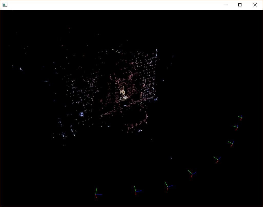
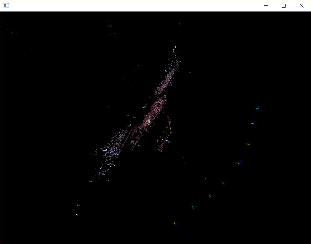
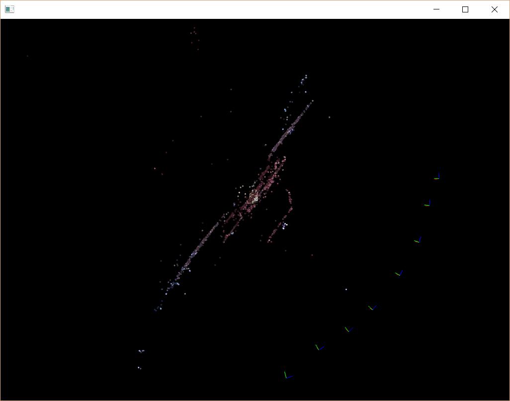
优化结果对比
Before

After
Before
After
Statistics
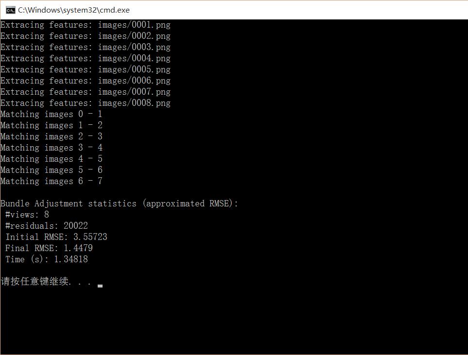
从统计信息可以看出,最初的重建结果,反向投影误差约为3.6个像素,BA之后,反向投影误差降为1.4个像素,如果删除一些误差过大的点,再进行一次BA,反向投影误差往往能小于0.5个像素!
这次的代码与上一篇文章的几乎一样,唯独多出来的几个函数和修改也已在上文中列出,这次就不再单独提供代码了。要运行本文的代码,需要编译Ceres Solver,还需要依赖Eigen(一个线性代数库),详细过程在Ceres的官网上均有提及。
结语
由于个人时间有限,马上就要面临毕业论文和工作等问题,这可能是该系列最后一篇文章。在此感谢各位朋友的支持,谢谢。


 本文介绍如何利用Ceres Solver实现三维重建中的Bundle Adjustment优化,通过反向投影误差的最小化提升重建精度。


 518
518

 被折叠的 条评论
为什么被折叠?
被折叠的 条评论
为什么被折叠?
 到【灌水乐园】发言


