


一、简介
论文链接:点击此链接查看HiDDeN的文献
JPEG压缩在HiDDeN网络的Noise Layer中,是通过近似模拟来实现的。
二、JPEG压缩流程
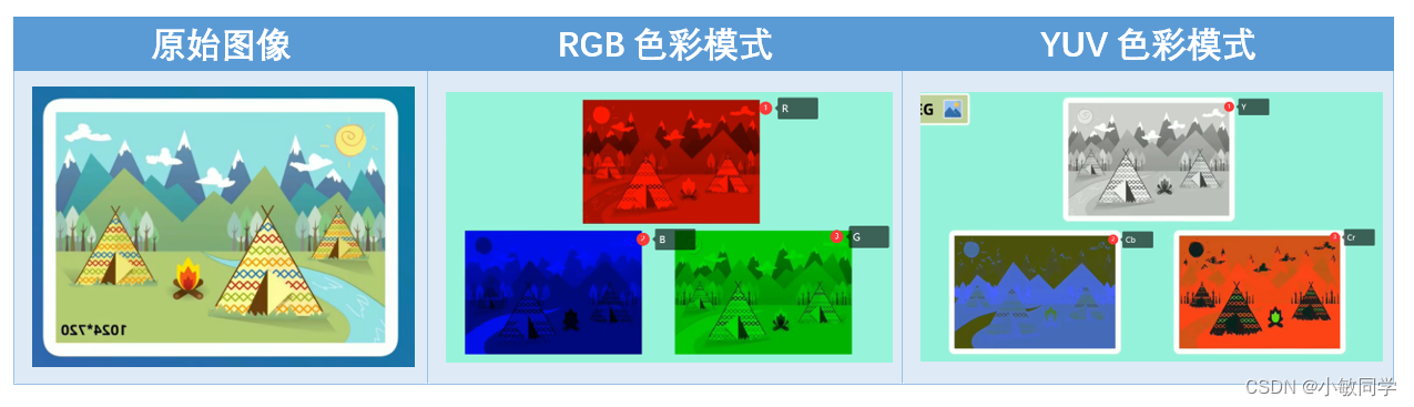
Step 1: 颜色模式转换。
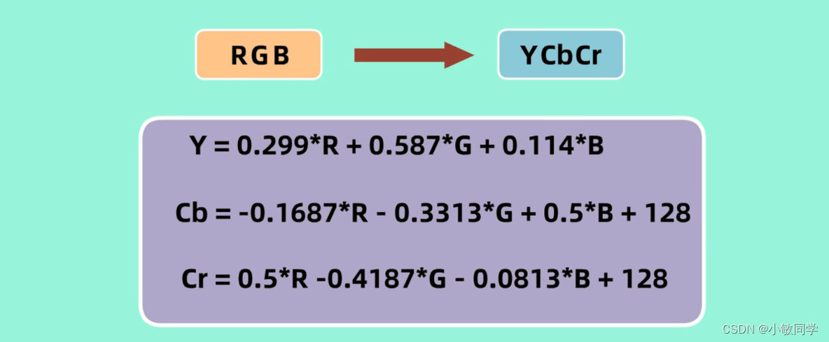
将RGB颜色空间,转化为YCbCr颜色空间。
RGB 通过红、绿、蓝三个颜色通道来表达颜色;
YCbCr 通过亮度、彩度蓝、彩度红三个通道来表达颜色;
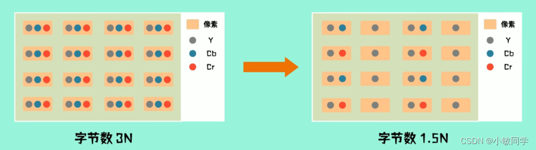
Step2 :向下采样。
在RGB颜色空间中,人眼对红、绿、蓝三种颜色的感知程度基本相当;
但是,在YUV颜色空间中,人眼对亮度的变化非常敏感,对色度的变化不易察觉;
因此,在下采样过程中,可以选择性的只保留一部分色度信息,从而达到减少数据量的效果。
常采用的采样方式 :
Y : U : V = 4 : 1 : 1( 每4个像素点保留1个彩度蓝、彩度红 );如下图所示,采样后的数据量减少了一半;
Y : U : V = 4 : 2 : 2 ( 每4个像素点保留2个彩度蓝、彩度红 );
补充说明: 没有被采样到的像素值,会用已采样到的邻近像素的值进行填充。具体来说,在每4x1的区域内,仅保留第一个像素的U值和V值,其余的三个像素的U值和V值被舍弃。
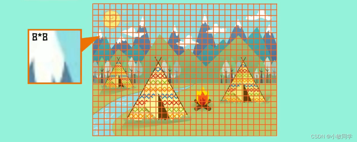
Step 3:8×8分块。
在DCT变换之前,需要将图像分为8*8的块。
因为DCT是基于8*8的图像块进行变换的。
若图像的宽、高不是8的倍数,需要对图像的宽、高进行填充。
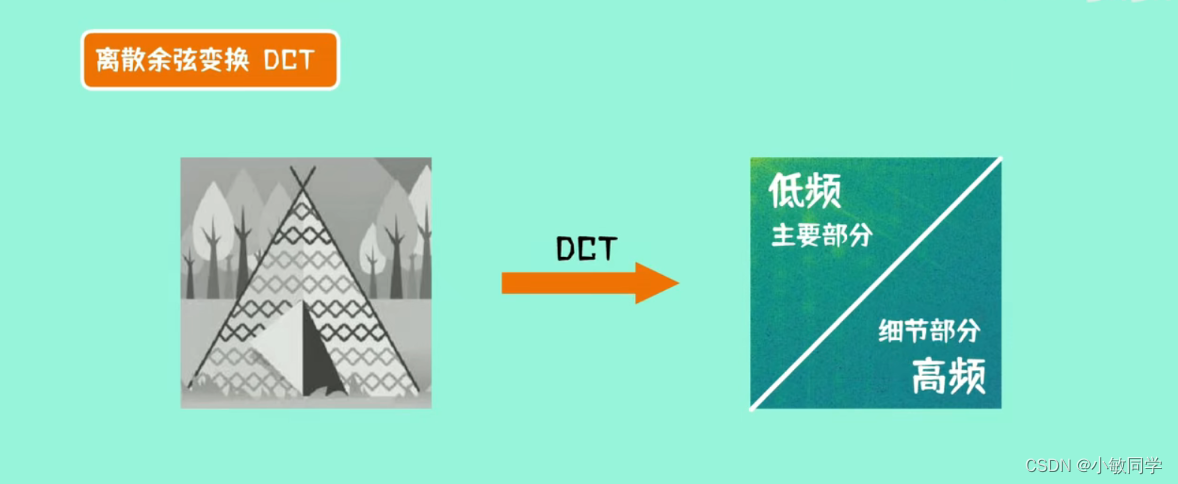
Step 4:离散余弦变换。
根据冈萨雷斯的《数字图像处理》可知:一切信号都可以用若干不同频率的标准余弦信号通过特定的组合形式表示出来,从而形成频域编码。
DCT变换的目的: 图像块经过离散余弦变换之后,低频部分集中在左上部分;高频部分集中在图片的右下部分,如下图所示。其中,低频部分是图片的主要内容,涵盖了图像的大部分信息;高频部分是图片的细节,人眼对这部分信息的失真并不敏感。因此,可以丢弃掉这部分信息,进一步减小数据量。
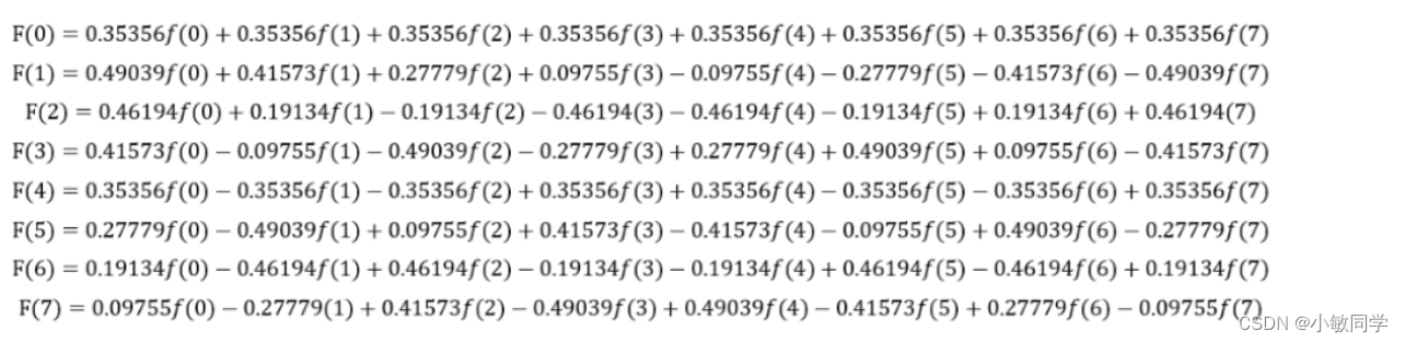
一维离散余弦变换的公式:

其中,F(u)是余弦变换后的值,u∈(0, 1, 2, …, N-1)。N表示信号的长度。f(x)是原始值,x∈(0, 1, 2, …, N-1)。当u=0时,𝐶𝑢 = 1⁄√2;其它情况下,𝐶𝑢 =1。
若要对一个长度为8的一维向量 [f(0), f(1), f(2), f(3), f(4), f(5), f(6), f(7)] 进行离散余弦变换,
根据上面的公式,将变换系数展开可得:

所以,将u=(0, 1, 2, …, 7)带入上式,可算得一维1×8向量的离散余弦变换的结果F(u):
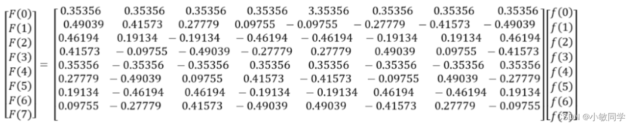
将其写成矩阵的形式,可以表示为:
一维1*8的块,对应的离散余弦变换系数的代码,如下所示:
import math
import numpy as np
import pandas as pd

# 一维离散余弦变换
def dct_coeff(x, u, N):
    if u == 0:
        return math.sqrt(1 / N)
    else:
        return math.sqrt(2 / N) * math.cos((math.pi * (2 * x + 1) * u) / (2 * N))


# 计算信号的DCT系数
dct_coeffs = []
for u in range(8):
    for x in range(8):
        dct_coeffs.append(dct_coeff(x, u, 8))

dct_coeffs = np.array(dct_coeffs).reshape((8, 8))
print("dct_coeffs: \n", dct_coeffs)
二维离散余弦变换的公式:
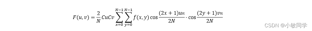
其中,F(u,v)是余弦变换后的值,u,v∈(0, 1, 2, …, N-1)。N表示信号的长度。f(x,y)是原始值,x,y∈(0, 1, 2, …, N-1)。当 𝑢 = 𝑣=0 时,𝐶𝑢 = 𝐶𝑣 = 1⁄√2;其它情况下,𝐶𝑢 = 𝐶𝑣 =1。
若要对一个8×8的二维向量进行离散余弦变换,根据上面的公式,将变换系数展开可得:
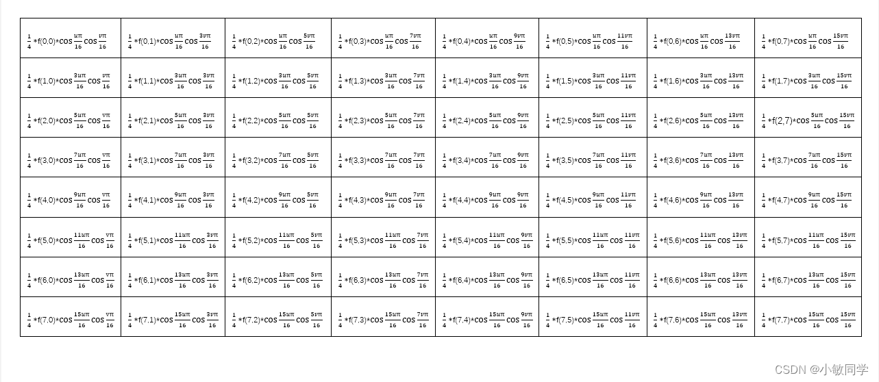
所以,将u,v=(0, 1, 2, …, 7)带入上式,可算得二维8×8向量的离散余弦变换的结果F(u),即64个8×8的二维表格。
二维8*8的块,对应的离散余弦变换系数的代码,如下所示:
import math
import numpy as np
import pandas as pd

# 计算信号的二维DCT系数
dct_coeffs_2d = []
for v in range(8):
    for u in range(8):
        for y in range(8):
            for x in range(8):
                # 将系数添加到dct_coeffs_2d中
                dct_coeffs_2d.append(dct_coeff_2d(x, y, u, v, 8))

# 将1个8x8的二维DCT系数矩阵转换为1个64x1的一维DCT系数矩阵
dct_coeffs_2d = np.array(dct_coeffs_2d).reshape((64, 64))
df = pd.DataFrame(dct_coeffs_2d)
df.to_excel("dct_coeffs_2d.xlsx")
DCT离散余弦变换的其它形式,详情见:点击此链接查看DCT变换的多种形式
Step 5:量化
量化的过程,就是丢弃信息的过程(丢弃信息的过程,其实就是减小数据量的过程)。
人眼对色彩的敏感要低于亮度,因此,对于Y和CrCb,定义了不同的量化系数。量化表格(质量因子Q=50)如下所示:
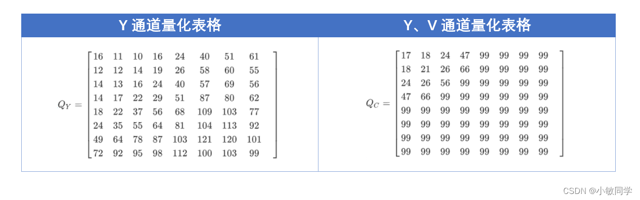
补充说明: 在JPEG压缩过程中,不同的质量因子会使用不同的量化表。通常,质量因子越高,量化表中的数值越小,图像的细节保留得越好,图像质量也就越高。而质量因子越低,量化表中的数值越大,图像的细节被压缩得更多,图像质量也就越低。
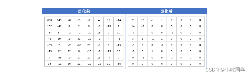
量化是有损的操作,经过量化后的系数矩阵中,右下部分出现大量的0。这对后续的编码操作来说是非常有利的。对一个8*8的图像块的Y通道采用以上Y通道量化表,量化后的结果如下所示:
Step 6:zigzag扫描
对量化后的矩阵进行之字化扫描,具体扫描过程如下:
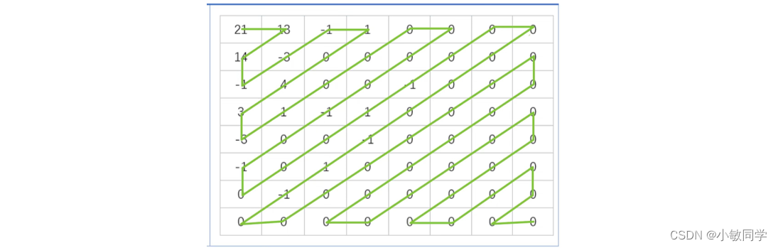
扫描以后的内容为:
21, 13, 14, -1, -3, -1, 1, 0, 4, 3, -3, 1, 0, 0, 0, 0, 0, 0, -1, 0, -1, 0, 0, 0, 1, -1, 0, 0, 0, 0, 0, 0, -1, 1, -1, 0, 0, 0, 0, 0, …
可以看到,0在很多位置连续出现。
Step 7:熵编码
对压缩信息进行huffman编码处理,具体操作流程见:JPEG压缩Huffman编码部分
参考资料列表:
[1] JPEG压缩视频介绍:点击此链接查看JPEG压缩的视频解说
[2] JPEG图像压缩原理:点击此链接查看JPEG图像压缩原理
[3] JPEG图像压缩算法流程详解:点击此链接查看JPEG图像压缩算法流程详解
[4] JPEG图像压缩算法:点击此链接查看JPEG图像压缩算法
[5] 二维离散余弦变换:点击此链接查看二维DCT变换过程
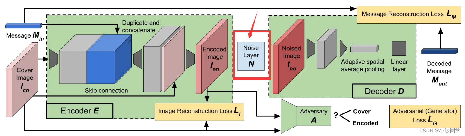
三、HiDDeN的JPEG压缩模块
3.1 难点分析
上述JPEG压缩的流程图,如下所示:

根据以上流程,逐一进行分析,可得:
-
颜色模式转换,通过公式即可完成。
-
向下采样,在HiDDeN的代码中没有出现。
-
8×8分块,通过reshape函数即可完成。
-
离散余弦变换,算得离散余弦变换系数,通过卷积即可完成。具体采用大小为8 × 8的64个filter,stride为8进行卷积实现DCT变换,每个filter对应于DCT变换中的一个基向量。
-
量化。论文中提到:JPEG压缩的量化步骤是不可微的,无法直接应用于梯度优化的训练中。为了解决这个问题,该论文中采用了可微的近似方法来模拟JPEG压缩的量化效果。
量化为什么是不可微的?
在DNN中,量化通常是将浮点数值除以量化矩阵并将结果四舍五入到最接近的整数。量化之后的四舍五入操作是不可微的,因为它是一个不连续的、分段常数的函数,导致在梯度反向传播时无法求导。因此,为了在DNN中使用量化,需要寻找可微分的近似方法。
可微和梯度优化之间的关系?
梯度优化的过程可以分为以下几步:
- 随机初始化模型参数。初始参数可以是任意值,但通常是一个随机的小数值,以避免算法陷入局部最优解。
- 计算损失函数对参数的梯度。梯度是损失函数关于每个参数的导数 ,它描述了损失函数随着参数变化的速度和方向。这里使用链式法则来计算梯度。
- 根据梯度更新模型参数。更新参数的方式是将当前参数减去梯度乘以一个学习率的大小。
- 重复步骤2-3,直到损失函数达到最小值或者达到算法停止的条件。
3.2 解决方法
论文主要思想:作者认为量化等同于限制通过该“通道”传输的信息量。
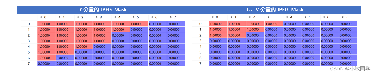
因此,使用JPEG-Mask将固定的一组高频系数清零。
具体而言,每个8×8的Y分量保留25个系数,U和V分量保留9个系数,如下所示:
补充说明:量化之后的步骤都是可逆操作,所以,JPEG压缩的模拟到此结束。然后,对图像进行逆变换(IDCT变换、YUV → RGB、去除填充),实现解压缩。
3.3 JPEG压缩具体代码
JPEG compression模块的代码,如下所示:
import numpy as np
import torch
import torch.nn as nn
import torch.nn.functional as F
from PIL import Image
from torchvision import datasets, transforms


def dct_coeff(n, k, N):
    # 该函数返回一个值,表示离散余弦变换(Discrete Cosine Transform,DCT)中的一个系数。
    return np.cos(np.pi / N * (n + 1. / 2.) * k)


def idct_coeff(n, k, N):
    # 该函数返回一个值,表示离散余弦逆变换(Inverse Discrete Cosine Transform,IDCT)中的一个系数。
    return (int(0 == n) * (- 1 / 2) + np.cos(
        np.pi / N * (k + 1. / 2.) * n)) * np.sqrt(1 / (2. * N))


def gen_filters(size_x: int, size_y: int, dct_or_idct_fun: callable) -> np.ndarray:
    tile_size_x = 8
    filters = np.zeros((size_x * size_y, size_x, size_y))
    for k_y in range(size_y):
        for k_x in range(size_x):
            for n_y in range(size_y):
                for n_x in range(size_x):
                    filters[k_y * tile_size_x + k_x, n_y, n_x] = dct_or_idct_fun(n_y, k_y, size_y) * dct_or_idct_fun(
                        n_x,
                        k_x,
                        size_x)
    return filters


def rgb2yuv(image_rgb, image_yuv_out):
    """ Transform the image from rgb to yuv """
    image_yuv_out[:, 0, :, :] = 0.299 * image_rgb[:, 0, :, :].clone() + 0.587 * image_rgb[:, 1, :,
                                                                                :].clone() + 0.114 * image_rgb[:, 2, :,
                                                                                                     :].clone()
    image_yuv_out[:, 1, :, :] = -0.14713 * image_rgb[:, 0, :, :].clone() + -0.28886 * image_rgb[:, 1, :,
                                                                                      :].clone() + 0.436 * image_rgb[:,
                                                                                                           2, :,
                                                                                                           :].clone()
    image_yuv_out[:, 2, :, :] = 0.615 * image_rgb[:, 0, :, :].clone() + -0.51499 * image_rgb[:, 1, :,
                                                                                   :].clone() + -0.10001 * image_rgb[:,
                                                                                                           2, :,
                                                                                                           :].clone()


def yuv2rgb(image_yuv, image_rgb_out):
    """ Transform the image from yuv to rgb """
    image_rgb_out[:, 0, :, :] = image_yuv[:, 0, :, :].clone() + 1.13983 * image_yuv[:, 2, :, :].clone()
    image_rgb_out[:, 1, :, :] = image_yuv[:, 0, :, :].clone() + -0.39465 * image_yuv[:, 1, :,
                                                                           :].clone() + -0.58060 * image_yuv[:, 2, :,
                                                                                                   :].clone()
    image_rgb_out[:, 2, :, :] = image_yuv[:, 0, :, :].clone() + 2.03211 * image_yuv[:, 1, :, :].clone()


def get_jpeg_yuv_filter_mask(image_shape: tuple, window_size: int, keep_count: int):
    mask = np.zeros((window_size, window_size), dtype=np.uint8)

    index_order = sorted(((x, y) for x in range(window_size) for y in range(window_size)),
                         key=lambda p: (p[0] + p[1], -p[1] if (p[0] + p[1]) % 2 else p[1]))

    for i, j in index_order[0:keep_count]:
        mask[i, j] = 1

    return np.tile(mask, (int(np.ceil(image_shape[0] / window_size)),
                          int(np.ceil(image_shape[1] / window_size))))[0: image_shape[0], 0: image_shape[1]]


class JpegCompression(nn.Module):
    def __init__(self, device, yuv_keep_weights=(25, 9, 9)):
        super(JpegCompression, self).__init__()
        self.device = device
        self.yuv_keep_weights = yuv_keep_weights
        self.dct_conv_weights = torch.tensor(gen_filters(8, 8, dct_coeff), dtype=torch.float32).to(self.device)
        self.dct_conv_weights.unsqueeze_(1)
        self.idct_conv_weights = torch.tensor(gen_filters(8, 8, idct_coeff), dtype=torch.float32).to(self.device)
        self.idct_conv_weights.unsqueeze_(1)
        self.jpeg_mask = None
        self.create_mask((1000, 1000))

    def create_mask(self, requested_shape):
        if self.jpeg_mask is None or requested_shape > self.jpeg_mask.shape[1:]:
            self.jpeg_mask = torch.empty((3,) + requested_shape, device=self.device)
            for channel, weights_to_keep in enumerate(self.yuv_keep_weights):
                mask = torch.from_numpy(get_jpeg_yuv_filter_mask(requested_shape, 8, weights_to_keep))
                self.jpeg_mask[channel] = mask

    def get_mask(self, image_shape):
        # if the mask is too small, create a new one
        if self.jpeg_mask.shape < image_shape:
            self.create_mask(image_shape)
        return self.jpeg_mask[:, :image_shape[1], :image_shape[2]].clone()

    def apply_conv(self, image, filter_type: str):

        if filter_type == 'dct':
            filters = self.dct_conv_weights
        elif filter_type == 'idct':
            filters = self.idct_conv_weights
        else:
            raise ('Unknown filter_type value.')

        image_conv_channels = []
        for channel in range(image.shape[1]):
            image_yuv_ch = image[:, channel, :, :].unsqueeze_(1)  # add channel dimension
            image_conv = F.conv2d(image_yuv_ch, filters, stride=8)
            image_conv = image_conv.permute(0, 2, 3, 1)
            image_conv = image_conv.view(image_conv.shape[0], image_conv.shape[1], image_conv.shape[2], 8, 8)
            image_conv = image_conv.permute(0, 1, 3, 2, 4)
            image_conv = image_conv.contiguous().view(image_conv.shape[0],
                                                      image_conv.shape[1] * image_conv.shape[2],
                                                      image_conv.shape[3] * image_conv.shape[4])

            image_conv.unsqueeze_(1)  # add channel dimension
            image_conv_channels.append(image_conv)
        image_conv_stacked = torch.cat(image_conv_channels, dim=1)  # stack channels
        return image_conv_stacked

    def forward(self, img):
        # 1. 对图片进行预处理(长、宽补充为8的倍数)
        noised_image = img
        # pad the image so that we can do dct on 8x8 blocks
        pad_height = (8 - noised_image.shape[2] % 8) % 8
        pad_width = (8 - noised_image.shape[3] % 8) % 8
        noised_image = nn.ZeroPad2d((0, pad_width, 0, pad_height))(noised_image)

        # 2. 将图片转换为YUV颜色空间
        image_yuv = torch.empty_like(noised_image)
        rgb2yuv(noised_image, image_yuv)

        # 3. 对图片进行DCT变换
        image_dct = self.apply_conv(image_yuv, 'dct')

        # 4. 对图片进行量化
        mask = self.get_mask(image_dct.shape[1:])
        image_dct_mask = torch.mul(image_dct, mask)

        # 5. 对图片进行反DCT变换
        image_idct = self.apply_conv(image_dct_mask, 'idct')

        # 6. 将图片转换为RGB颜色空间
        image_ret_padded = torch.empty_like(image_dct)
        yuv2rgb(image_idct, image_ret_padded)

        # 7. 将图片去除预处理的补充部分
        img = image_ret_padded[:, :, :image_ret_padded.shape[2] - pad_height,
              :image_ret_padded.shape[3] - pad_width].clone()

        return img


# 调用以上代码
device = torch.device("cpu")
# noised_image = torch.randn(1, 3, 128, 128)
# 读取一张本地图片
img = Image.open("E:\EXPERIMENT\study\hidden_my\data\cover.jpg")
# 将图片转换为tensor
noised_image = transforms.ToTensor()(img)
# 将图片添加一个维度
noised_image = noised_image.unsqueeze(0)
JpegCompression(device, yuv_keep_weights=(25, 9, 9))(noised_image)
四、其它噪声模块
其它噪声模块的解释:点击此链接查看其它噪声模块详解
  (noiser): Noiser(
    (noise_layers): Sequential(
      (0): Identity()
      (1): Crop()
      (2): Cropout()
      (3): Dropout()
      (4): Resize()
      (5): Gaussian()
      (6): JpegCompression()
    )


 8万+
8万+

 被折叠的 条评论
为什么被折叠?
被折叠的 条评论
为什么被折叠?
 到【灌水乐园】发言


