


一、简介
论文链接:点击此链接查看RedMark的文献
论文中的Encoder结构,如下图所示:
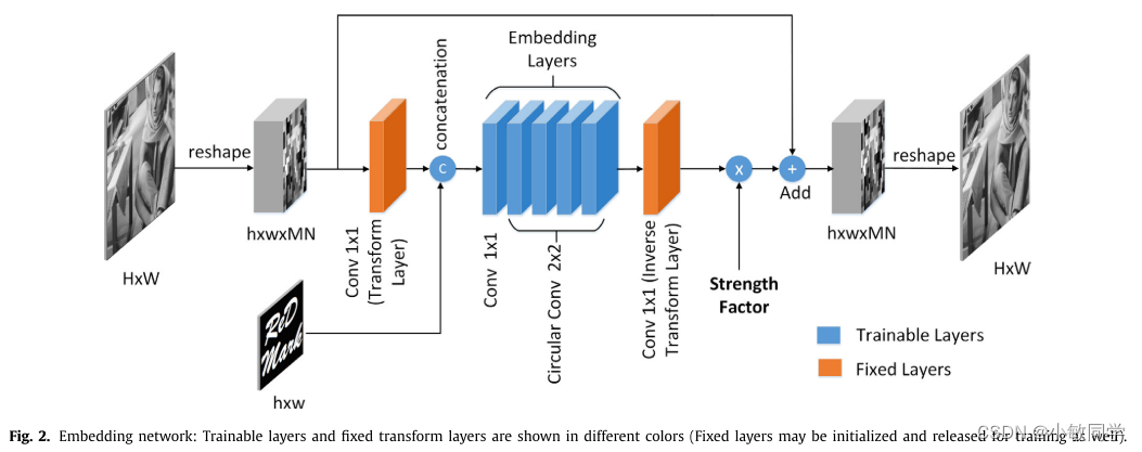
Encoder功能: 将16bit消息串嵌入到宿主图像中,形成编码图像
Encoder输入1: Cover Image(宿主图像) = 32×32×1
Encoder输入2: Message(随机二进制bit) = 16bit
Encoder输出: Encoded Image(编码图像) = 32×32×1
Encoder实现流程:
- Reshape,将(n, 32, 32, 1)的图像变为(n, 4, 4, 64);其中,n表示batch size;
- 变换,将图像从空域转到变换域;论文中主要采用的是DCT域;
- 连接,将频域图像与水印连接到一起;
- 卷积,1次普通2D卷积 + 4次循环卷积;其中,循环卷积是作者自己定义的模块;
- 逆变换,将图像从变换域转回空域;
- 嵌入,将第5步的结果 × 嵌入强度因子 + 宿主图像,得到编码图像;
- 逆Reshape,得到编码图像,将其变为(n, 32, 32, 1);
二、编码器模块
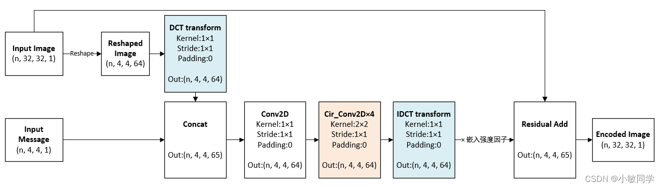
2.1 整体模块
RedMark的整个编码网络的具体结构图如下所示:
RedMark的整个编码网络的具体代码如下所示:
from tensorflow.keras import layers
import tensorflow as tf
import numpy as np
import scipy.io as sio
from include.my_circular_layer import Conv2D_circular

# 1. Load input image
input_img = layers.Input(shape=(32, 32, 1), name='input_img')
print("input_img.shape", input_img.shape)

# 2. Rearrange input image
rearranged_img = l1 = layers.Lambda(tf.space_to_depth, arguments={'block_size': 8}, name='rearrange_img')(
    input_img)
print("rearranged_img.shape", rearranged_img.shape)

# 3. use DCT to transform the input image
dct_layer = layers.Conv2D(64, (1, 1), activation='linear', input_shape=(4, 4, 64), padding='same', use_bias=False,
                          trainable=False, name='dct')
dct_layer_img = dct_layer(rearranged_img)
print("dct_layer_img.shape", dct_layer_img.shape)  # (1, 4, 4, 64)

# 4. Define watermark
input_watermark = layers.Input(shape=(4, 4, 1), name='input_watermark')
print("input_watermark.shape", input_watermark.shape)  # (None, 4, 4, 1)

# 5. Concatenating The Image's dct coefs and watermark
encoder_input = layers.Concatenate(axis=-1, name='encoder_input')([dct_layer_img, input_watermark])
print("encoder_input.shape", encoder_input.shape)  # (1, 4, 4, 65)


# 6. Encoder
encoder_model = layers.Conv2D(64, (1, 1), dilation_rate=1, activation='elu', padding='same',
                              name='enc_conv1')(encoder_input)
encoder_model = Conv2D_circular(64, (2, 2), dilation_rate=1, activation='elu', padding='same',
                                name='enc_conv2')(encoder_model)
encoder_model = Conv2D_circular(64, (2, 2), dilation_rate=1, activation='elu', padding='same',
                                name='enc_conv3')(encoder_model)
encoder_model = Conv2D_circular(64, (2, 2), dilation_rate=1, activation='elu', padding='same',
                                name='enc_conv4')(encoder_model)
encoder_model = Conv2D_circular(64, (2, 2), dilation_rate=1, activation='elu', padding='same',
                                name='enc_conv5')(encoder_model)
idct_layer = layers.Conv2D(64, (1, 1), activation='linear', input_shape=(4, 4, 64), padding='same', use_bias=False,
                           trainable=False, name='idct')
encoder_model = idct_layer(encoder_model)
encoder_model = layers.Add(name='residual_add')([encoder_model, l1])

# 7. Rearrange the output
x = layers.Lambda(tf.depth_to_space, arguments={'block_size': 8}, name='enc_output_depth2space')(encoder_model)
print("encoder_output:", x.shape)

# 8. Define the model
model = tf.keras.models.Model(inputs=[input_img, input_watermark], outputs=x)

# 9. Set IDCT coefficients
idct_mtx = sio.loadmat('./weights/IDCT_coef.mat')['IDCT_coef']
idct_mtx = np.reshape(idct_mtx, [1, 1, 64, 64])
model.get_layer('idct').set_weights(np.array([idct_mtx]))

# 10. Set DCT coefficients
dct_mtx = sio.loadmat('./weights/DCT_coef.mat')['DCT_coef']
dct_mtx = np.reshape(dct_mtx, [1, 1, 64, 64])
model.get_layer('dct').set_weights(np.array([dct_mtx]))
2.2 DCT变换层
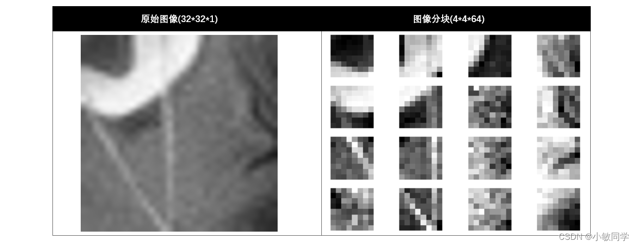
2.2.1 分块
因为DCT变换是对8×8的图像块进行的,所以在DCT变换之前,需要把图像分为n个8×8的块。
具体的,通过tf.nn.space_to_depth函数实现分块,代码如下:
import tensorflow as tf
import matplotlib.pyplot as plt
from tensorflow.keras import layers
from PIL import Image

input_img = Image.open('images/img/img (1).jpg')
input_img = tf.convert_to_tensor(input_img, dtype=tf.float32)
input_img = tf.reshape(input_img, [1, 32, 32, 1])

rearranged_img = layers.Lambda(tf.nn.space_to_depth, arguments={'block_size': 8}, name='rearrange_img')(
    input_img)

for i in range(4):
    for j in range(4):
        block = rearranged_img[0, i, j]
        block = tf.reshape(block, [8, 8])
        plt.subplot(4, 4, i * 4 + j + 1)
        plt.imshow(block, cmap='gray')
        plt.axis('off')
plt.show()
将32×32的图像,分为16个8×8大小的块,结果如下所示:
2.2.2 DCT变换
DCT变换可以简单理解为把原始图像块与DCT变换系数矩阵相加乘,这一过程在网络中可以通过卷积层实现。特别地,需要将该层的权重系数设置为固定的二维DCT系数矩阵(64×64),代码如下所示:
from tensorflow.keras import layers
import tensorflow as tf
import numpy as np
import scipy.io as sio
from PIL import Image
import matplotlib.pyplot as plt

# 1. Load input image
img = Image.open('./images/img/img (1).jpg').convert('L')
input_img = tf.convert_to_tensor(img, dtype=tf.float32)
input_img = tf.reshape(input_img, [1, 32, 32, 1])

# 2. Rearrange input nx32x32x1 -> nx4x4x64(8×8)
rearranged_img = l1 = layers.Lambda(tf.nn.space_to_depth, arguments={'block_size': 8}, name='rearrange_img')(
    input_img)

# 3. Define the model
model = tf.keras.models.Sequential()
model.add(
    tf.keras.layers.Conv2D(64, (1, 1), activation='linear', input_shape=(4, 4, 64), padding='same', use_bias=False,
                           trainable=False, name='dct'))

# 4. Set DCT coefficients
dct_mtx = sio.loadmat('transforms/DCT_coef.mat')['DCT_coef']
dct_mtx = np.reshape(dct_mtx, [1, 1, 64, 64])
model.get_layer('dct').set_weights(np.array([dct_mtx]))

# 5. Apply the model to the input image
output_img = model.predict(rearranged_img, steps=1)

# 5. Show the output image
for i in range(4):
    for j in range(4):
        block = output_img[0, i, j]
        block = tf.reshape(block, [8, 8])
        print("block i", i, "j", j, ":", block)
        plt.subplot(4, 4, i * 4 + j + 1)
        plt.imshow(block, cmap='gray')
        plt.axis('off')
plt.show()
经过DCT变换之后,得到了每个图像块的频域结果:
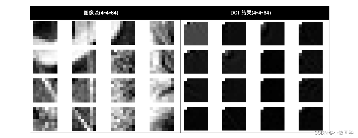
由以上图片可见,经过DCT变换之后,每个图像块的低频部分被集中到左上角,高频部分被集中于右下角。
2.3 循环卷积层
循环卷积的功能: 使用循环卷积避免零填充,提高水印质量和鲁棒性。使得水印在图像边界上得到进一步扩散和数据共享(所有的神经元平等地共享水印数据),从而避免零填充导致的水印质量下降效应。
循环卷积的实现方式: 重写Tensorflow框架的tf.keras.layers.Conv2D方法,改变卷积过程中的padding,不采用0填充,而是采用图像像素值填充。然后,封装成Conv2D_circular模块,以供定义编解码器的网络层时调用。
循环卷积的理解:
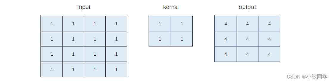
对于一个4×4的图像块,使用1×1的卷积核进行卷积,则会得到一个3×3的卷积结果,效果如下:
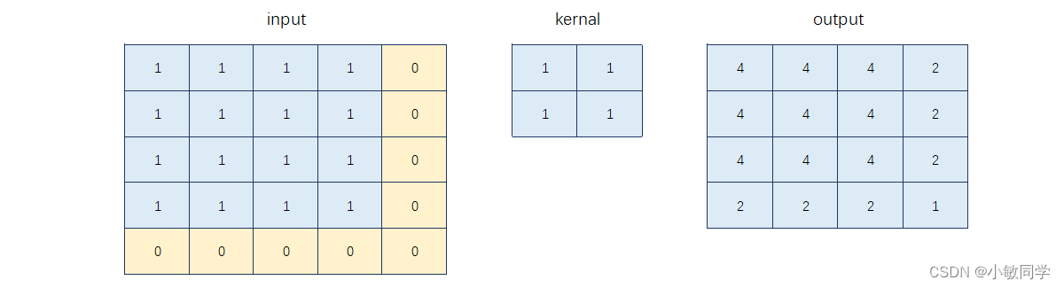
如果希望输出也是4×4,在卷积过程中,通过padding=same可以实现,默认填充0,效果如下:
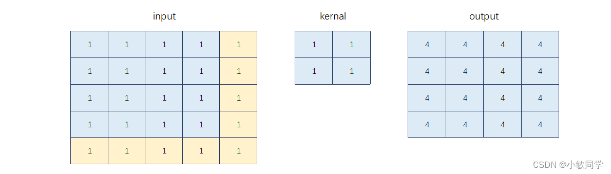
作者的目的是避免0填充,而是采用原始像素值进行填充,效果如下:


 58
58

 被折叠的 条评论
为什么被折叠?
被折叠的 条评论
为什么被折叠?
 到【灌水乐园】发言


