


注:md文件,Typora书写,md兼容程度github=CSDN>知乎,若有不兼容处麻烦移步其他平台,github文档供下载。
发表在CSDN:https://blog.csdn.net/hancoder/article/
发表在知乎专栏:https://zhuanlan.zhihu.com/c_1088438808227254272
上传在github:https://github.com/FermHan/Learning-Notes
SSD
SSD:Single Shot MultiBox Detector
作者:Wei Liu
前言
背景知识:faster rcnn与YOLO,不熟悉可参考本人csdn。
faster rcnn发展史:https://blog.csdn.net/hancoder/article/details/87917174 。
YOLO:https://blog.csdn.net/hancoder/article/details/87994678 ,知乎专栏也有。
标题解释:SSD:Single Shot MultiBox Detector
Single shot:SSD是one-stage方法,单阶段表示定位目标和分类的任务是在网络的一次前向传递中完成的。而faster rcnn是双阶段的,先通过CNN得到候选框roi,然后再进行分类与回归。
MultiBox:SSD是多框预测。
Detector:物体检测器,并分类
在faster rcnn中,anchors只作用在最后的conv5_3的特征图上,这对检测小物体及位置来说是有不足的,所以SSD想在多个特征图上用anchors回归检测物体。高层特征图的语义信息丰富对分类有益,而低层特征图语义信息少但位置信息多,利于定位。
SSD有多好:速度与mAP对比:
SSD:59 FPS with mAP 74.3% on VOC2007 test,
Faster R-CNN: 7 FPS with mAP 73.2%
YOLO: 45 FPS with mAP 63.4%
框架介绍
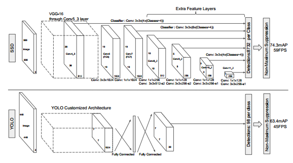
如图,下半部分是YOLO的结果,他只利用conv5特征图进行回归分类来目标检测。缺点:小目标丢失,位置信息有丢失。
结构图的上半部分是SSD采样金字塔结构,综合conv4_3、conv7、conv8_2、conv9_2、conv10_2、conv11_2这些层的feature map进行目标检测,同时进行softmax分类和位置回归。图上用的是1个3×3整体卷积出来位置与分类,代码里是2个3×3分别卷积,whatever,原理都一样这也不是重点。加入了先验框。
什么是金字塔结构:这里无需复杂理解,只知道它如上图结构图那样,经过池化后图像逐渐缩小即可。想进一步阅读比SSD更复杂的金字塔结构可以参考本人FPN博客:https://blog.csdn.net/hancoder/article/details/89048870
SSD创新点
单阶段
YOLOv1也是单阶段,但SSD比YOLO快还准。
多特征图上预测
YOLO主要利用conv5_3上的信息进行预测,而SSD利用了多个特征图:conv4_3、conv7、conv8_2、conv9_2、conv10_2、conv11_2。
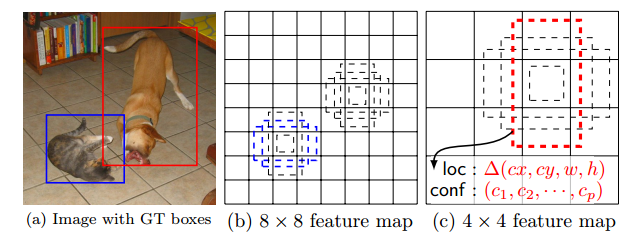
划分特征图
r如果是YOLO,会把特征图均分成7×7,分割后的每个小块叫一个cell单元,然后以每个cell单元为中心,像faster rcnn那样,预设一些anchors。不同的是SSD中把anchors锚称作了priors或default boxes,而且SSD因为在很后面的特征图上操作,所以是以每个像素为单位划分的。
prior的具体设置如下
| 特征图 | feature_size | prior_per_cell | Total_num |
|---|---|---|---|
| conv4_3 | 38×38 | 4 | 5776 |
| conv7 | 19×19 | 6 | 2166 |
| conv8_2 | 10×10 | 6 | 600 |
| conv9_2 | 5×5 | 6 | 150 |
| conv10_2 | 3×3 | 4 | 36 |
| conv11_2 | 1×1 | 4 | 4 |
| 输入300×300 | 总和对应的即图上的8732 | 8732 |
此外,因为faster rcnn中是在单个特征图conv5_3上放置anchors,所以anchors所在特征图相对原图的比例是不变的,都是1/16。所以faster rcnn的scale统一定3个值即可。但是SSD是在多个特征图上进行的,所以后文我们需要介绍在不同特征图上的priors的scale是如何定义的。
prior的scale与ratio
下面来看下SSD选择anchor的方法。首先每个点cell都会有一大一小两个正方形的anchor,小方形的边长用min_size来表示,大方形的边长用sqrt(min_size*max_size)来表示(min_size与max_size的值每一层都不同)。同时还有多个长方形的anchor,长方形anchor的数目在不同层级会有差异,他们的长宽可以用下面的公式来表达,ratio的数目就决定了某层上每一个点对应的长方形anchor的数目。
在faster rcnn中有scale和ratio两个数值,而SSD中,每个feature map上的scale的算法是
s k = s m i n + s m a x − s m i n m − 1 ( k − 1 ) , k ∈ [ 1 , m ] s_k=s_{min}+ {{s_{max}-s_{min}}\over{m-1}}(k-1),k∈[1,m] sk=smin+m−1smax−smin(k−1),k∈[1,m]
m代表预测时feature map的数量,如SSD300的m=6,分别是conv4_3、conv7、conv8_2、conv9_2、conv10_2、conv11_2。
在faster rcnn中scale可能是一个具体的大小,SSD中代表的是相对输入图像的比例。
smax和smin代表最低层和最高层分别有scale:0.2和0.9。 s m i n = 0.2 , s m a x = 0.9 s_{min}=0.2,s_{max}=0.9 smin=0.2,smax=0.9。例如最高层回归出的每个基础框的尺寸大小是0.9×300=370。
第k层的min_size=Sk,第k层的max_size=Sk+1。(注意区分smin和min_size是不同的东西)
SSD按照如下规则生成prior box:
- 以feature map上每个点的中点为中心,生成N(4或6)个同心的prior box
- 两个正方形prior box变成分别为: m i n s i z e , m i n s i z e ∗ m a x s i z e minsize,\sqrt{minsize*maxsize} minsize,minsize∗maxsize,其中 m i n s i z e k = s k ∗ 300 , m a x s i z e k = s k + 1 ∗ 300 minsize_k=s_k*300 , maxsize_k=s_{k+1}*300 minsizek=sk∗300,maxsizek=sk+1∗300
- 此外还有4个正方形,长宽为: w i d t h = m i n s i z e × r a t i o , h e i t g h t = m i n s i z e × 1 / r a t i o width=minsize×\sqrt{ratio} , heitght=minsize×1/\sqrt{ratio} width=minsize×ratio,heitght=minsize×1/ratio,其中 r a t i o = { 2 , 3 , 1 / 2 , 1 / 3 } ratio=\{2,3,1/2,1/3\} ratio={2,3,1/2,1/3}。(论文中的1是正方形)
注:以上是作者论文中给的计算各层anchor尺寸的方法,但在作者源码中给的计算anchor方法有点差异,没有和论文的方法完全对应上。管他呢,反正这个东西都是超参数,差不多就行。
| 特征图 | min_size | max_size |
|---|---|---|
| conv4_3 | 30 | 60 |
| conv7 | 60 | 111 |
| conv8_2 | 111 | 162 |
| conv9_2 | 162 | 213 |
| conv10_2 | 213 | 264 |
| conv11_2 | 264 | 315 |
预设好anchoris后的如何卷积训练
如结构图,上半部分的横线上有3×3×(N×(classes+4))的字样(N为4或6),指的是在各个特征图上用3×3卷积,得出的通道数代表:每个cell预设了N个框,每个框有classes个类别,每个框有4个位置坐标信息。从这里我们也可以得知SSD与YOLOv1不同,SSD对于每个单元的每个先验框,其都输出一套独立的检测值,

训练与loss
给priors赋label
训练时每个框要有gt才能训练,即每个框要有label。关于给框赋label的操作我在我之前的论文Faster rcnn、FPN和YOLO中已多次提及了,这里简单引用一下我之前写的,赋label的原理都是一样的,不管是在RPN前背景分类还是在fast rcnn具体分类中。
RPN训练时需要有anchor的前背景类标。对anchor进行label的原理和Faster R-CNN里一模一样,详情可以去本人博客https://blog.csdn.net/hancoder/article/details/87917174 的RPNlabel部分查看。反正就是与gt的IoU>0.7就是正类label=1,IoU<0.3是负类背景label=0,其余介于0.3和0.7直接的都扔掉不参与训练label=-1。在faster rcnn中拿256个anchors训练后得到W×H×9个roi。
loss的计算:
SSD的loss和常规目标检测的loss一样:分类loss+位置回归loss
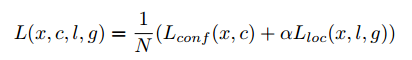
N是匹配的默认框的个数, α = 1 \alpha=1 α=1
confidence类别loss:采用交叉熵损失
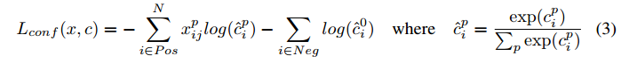
x i j p = 1 x_{ij}^p=1 xijp=1代表第i个default框与第j个真实框关于类别p相匹配,不匹配的 x i j p = 0 x_{ij}^p=0 xijp=0。前半个式子是pisitive,后半个是negative
根据上面的赋label策略,一定有 Σ i x i j p > = 1 \Sigma_ix_{ij}^p>=1 Σixijp>=1,这个式子的物体含义是任一编号为 j 的框gt,至少有1个默认框与其匹配,即每个gt框可能赋给了多个默认框。
SSD的类别是1背景+c个类别,1+c个置信度,第一个置信度指的是不含目标或者属于背景的评分。后面的c个累呗置信度其实包含1个背景,即实际类别c-1个,自己注意体会即可。置信度最高的类别即边框的类别。
location位置loss:
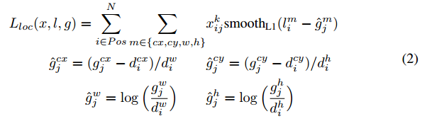
定位误差即fast rcnn里的smooth L1 loss,坐标分别算的是中心坐标与宽高。如果你大概看一眼,看就把l看作是预测的xywh,而g是真实的xywh。但不知你有没有想过如果只是这样直接回归,那默认框怎么在loss里体现?前面这种简单的回归方法在loss中只体现了预测值与真实值,但我们还有个默认框的先验值,我们是要在默认框上回归的。答案在于:如果你跑代码的话,你就会发现l和g分别是预测值和真实值这个说法虽然是正确的,但是l和g实际上分别是【预测框与默认框的距离】和【真实框和默认框的距离】,这样设置的话我们就把默认框的信息包含到loss里了。这种通过默认框间接得出预测框位置的方法的术语其实就是框信息的“编码解码”。这种编码方式文中叫做offset
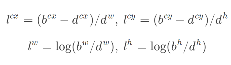
所以我再理解l和g的展开式就好理解了。编码前:d是默认default框 d = ( d c x , d c y , d w , d h ) d=(d^{cx},d^{cy},d^w,d^h) d=(dcx,dcy,dw,dh),预测框为 b = ( b c x , b c y , b w , b h ) b=(b^{cx},b^{cy},b^w,b^h) b=(bcx,bcy,bw,bh)。编码后:预测值是l=b-d。真实值是g^=g-d。为了归一化还除以了默认框的wh。
上面称为编码encode,预测后画框时我们需要反向这个过程,即进行解码decode,从预测值l中得到边界框的真实位置b
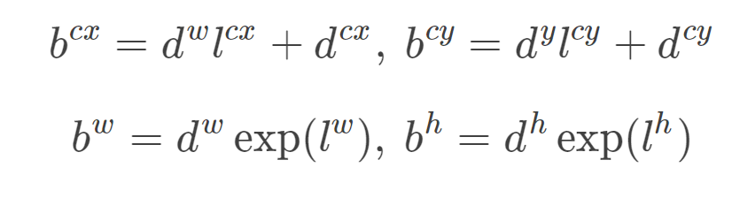
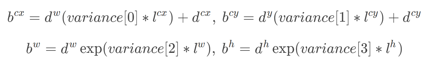
附别地方看到的一些内容:这个应该是caffe独有的内容?variance_encoded_in_target来控制两种模式,当其为True时,表示variance被包含在预测值中,就是上面那种情况。但是如果是Fasle(大部分采用这种方式,训练更容易?),就需要手动设置超参数variance,用来对ll的4个值进行放缩,此时边界框需要这样解码:
SSD的其他一些trick
Hard negative mining负样本挖掘
在生成一系列的 predictions 之后,会产生很多个符合 ground truth box 的 predictions boxes,但同时,不符合 ground truth boxes 也很多,而且这个 negative boxes,远多于 positive boxes。这会造成 negative boxes、positive boxes 之间的不均衡。训练时难以收敛。
解决措施:先随机抽取一定数目负框,然后排序抽得分高的若干个框。选择最高的几个,保证最后 negatives、positives 的比例在 3:1。

本文通过实验发现,这样的比例可以更快的优化,训练也更稳定。
Data augmentation数据增强
实验部分
a trous Algorithm
此部分内容借鉴了其他博客。
基于VGG16,预训练过。移除掉drpoout层和FC8,用SGD以0.001学习率,0.9动量,0.0005权重衰减,32batch size微调。
然后借鉴了DeepLab-LargeFOV,分别将VGG16的全连接层fc6和fc7转换成3×3卷积层conv6和1×1卷积层conv7,同时
将池化层pool5由原来的2×2−s2变成3×3−s1(猜想是不想reduce特征图大小),为了配合这种变化,采用了一种a trous Algorithm(hole filling algorithm),其实就是conv6采用扩展卷积或带孔卷积(Dilation Conv),其在不增加参数与模型复杂度的条件下指数级扩大卷积的视野,其使用扩张率(dilation rate)参数,来表示扩张的大小,如下图7所示,(a)是普通的3×3卷积,其视野就是3×3,(b)是扩张率为2,此时视野变成7×7,©扩张率为4时,视野扩大为15×15,但是视野的特征更稀疏了。Conv6采用3×3大小但dilation rate=6的扩展卷积。

另附两个关于a trous Algorithm(hole filling algorithm)的解读
博客 1:http://www.cnblogs.com/jianyingzhou/p/5386222.html
最早用的就是 deeplab 的文章了,Semantic Image Segmentation with Deep Convolutional Nets and Fully Connected CRFS 这篇文章和 fcn 不同的是,在最后产生 score map 时,不是进行upsampling,而是采用了 hole algorithm,就是在 pool4 和 pool 5层,步长由 2 变成 1,必然输出的 score map 变大了,但是 receptive field 也变小了,为了不降低 receptive field,怎么做呢?利用 hole algorithm,将卷积 weights 膨胀扩大,即原来卷积核是 3x3,膨胀后,可能变成 7x7 了,这样 receptive field 变大了,而 score map 也很大,即输出变成 dense 的了。
这么做的好处是,输出的 score map 变大了,即是 dense 的输出了,而且 receptive field 不会变小,而且可以变大。这对做分割、检测等工作非常重要。
博客 2:http://blog.csdn.net/tangwei2014/article/details/50453334
既想利用已经训练好的模型进行 fine-tuning,又想改变网络结构得到更加 dense 的 score map.
这个解决办法就是采用 Hole 算法。如下图 (a) (b) 所示,在以往的卷积或者 pooling 中,一个 filter 中相邻的权重作用在 feature map 上的位置都是物理上连续的。如下图 © 所示,为了保证感受野不发生变化,某一层的 stride 由 2 变为 1 以后,后面的层需要采用 hole 算法,具体来讲就是将连续的连接关系是根据 hole size 大小变成 skip 连接的(图 © 为了显示方便直接画在本层上了)。不要被 © 中的 padding 为 2 吓着了,其实 2 个 padding 不会同时和一个 filter 相连。
pool4 的 stride 由 2 变为 1,则紧接着的 conv5_1, conv5_2 和 conv5_3 中 hole size 为 2。接着 pool5 由 2 变为 1 , 则后面的 fc6 中 hole size 为 4。

Additional Notes On SSD
SSD的论文还作了以下的观察:
- 更多的default boxes会带来更精确的检测,但耗时增加
- 由于detector以多种分辨率运行于特征上,因此在多个图层上使用MultiBox也会导致更好的检测
- 80%的时间花在基础VGG-16网络上:这意味着,使用更快,同样精确的网络,SSD的性能可能会更好
- SSD将具有相似类别的对象(例如动物)混淆。这可能是因为定位是基于多个类的
- SSD-500(使用512x512输入图像的最高分辨率版本)在Pascal VOC2007上实现了最佳的mAP,达到了76.8%,但是速度降低到22 fps。因此SSD-300在59 fps下具有74.3 mAP更好的折衷。
- SSD在较小的对象上产生较差的性能,因为它们可能不会出现在所有功能地图中。增加输入图像分辨率缓解了这个问题,但并未完全解决这个问题
代码
keras代码地址:https://github.com/pierluigiferrari/ssd_keras/blob/master/models/keras_ssd300.py
代码只大概阅读,没有进行逐行研究,这里给出仅供参考。
基础网络
x = Input(shape=(img_height, img_width, img_channels))

# The following identity layer is only needed so that the subsequent lambda layers can be optional.
x1 = Lambda(identity_layer, output_shape=(img_height, img_width, img_channels), name='identity_layer')(x)
if not (subtract_mean is None):
x1 = Lambda(input_mean_normalization, output_shape=(img_height, img_width, img_channels), name='input_mean_normalization')(x1)
if not (divide_by_stddev is None):
x1 = Lambda(input_stddev_normalization, output_shape=(img_height, img_width, img_channels), name='input_stddev_normalization')(x1)
if swap_channels:
x1 = Lambda(input_channel_swap, output_shape=(img_height, img_width, img_channels), name='input_channel_swap')(x1)

conv1_1 = Conv2D(64, (3, 3), activation='relu', padding='same', kernel_initializer='he_normal', kernel_regularizer=l2(l2_reg), name='conv1_1')(x1)
conv1_2 = Conv2D(64, (3, 3), activation='relu', padding='same', kernel_initializer='he_normal', kernel_regularizer=l2(l2_reg), name='conv1_2')(conv1_1)
pool1 = MaxPooling2D(pool_size=(2, 2), strides=(2, 2), padding='same', name='pool1')(conv1_2)

conv2_1 = Conv2D(128, (3, 3), activation='relu', padding='same', kernel_initializer='he_normal', kernel_regularizer=l2(l2_reg), name='conv2_1')(pool1)
conv2_2 = Conv2D(128, (3, 3), activation='relu', padding='same', kernel_initializer='he_normal', kernel_regularizer=l2(l2_reg), name='conv2_2')(conv2_1)
pool2 = MaxPooling2D(pool_size=(2, 2), strides=(2, 2), padding='same', name='pool2')(conv2_2)

conv3_1 = Conv2D(256, (3, 3), activation='relu', padding='same', kernel_initializer='he_normal', kernel_regularizer=l2(l2_reg), name='conv3_1')(pool2)
conv3_2 = Conv2D(256, (3, 3), activation='relu', padding='same', kernel_initializer='he_normal', kernel_regularizer=l2(l2_reg), name='conv3_2')(conv3_1)
conv3_3 = Conv2D(256, (3, 3), activation='relu', padding='same', kernel_initializer='he_normal', kernel_regularizer=l2(l2_reg), name='conv3_3')(conv3_2)
pool3 = MaxPooling2D(pool_size=(2, 2), strides=(2, 2), padding='same', name='pool3')(conv3_3)

conv4_1 = Conv2D(512, (3, 3), activation='relu', padding='same', kernel_initializer='he_normal', kernel_regularizer=l2(l2_reg), name='conv4_1')(pool3)
conv4_2 = Conv2D(512, (3, 3), activation='relu', padding='same', kernel_initializer='he_normal', kernel_regularizer=l2(l2_reg), name='conv4_2')(conv4_1)
conv4_3 = Conv2D(512, (3, 3), activation='relu', padding='same', kernel_initializer='he_normal', kernel_regularizer=l2(l2_reg), name='conv4_3')(conv4_2)
pool4 = MaxPooling2D(pool_size=(2, 2), strides=(2, 2), padding='same', name='pool4')(conv4_3)

conv5_1 = Conv2D(512, (3, 3), activation='relu', padding='same', kernel_initializer='he_normal', kernel_regularizer=l2(l2_reg), name='conv5_1')(pool4)
conv5_2 = Conv2D(512, (3, 3), activation='relu', padding='same', kernel_initializer='he_normal', kernel_regularizer=l2(l2_reg), name='conv5_2')(conv5_1)
conv5_3 = Conv2D(512, (3, 3), activation='relu', padding='same', kernel_initializer='he_normal', kernel_regularizer=l2(l2_reg), name='conv5_3')(conv5_2)
pool5 = MaxPooling2D(pool_size=(3, 3), strides=(1, 1), padding='same', name='pool5')(conv5_3)
特征抽取
fc6 = Conv2D(1024, (3, 3), dilation_rate=(6, 6), activation='relu', padding='same', kernel_initializer='he_normal', kernel_regularizer=l2(l2_reg), name='fc6')(pool5)

fc7 = Conv2D(1024, (1, 1), activation='relu', padding='same', kernel_initializer='he_normal', kernel_regularizer=l2(l2_reg), name='fc7')(fc6)

conv6_1 = Conv2D(256, (1, 1), activation='relu', padding='same', kernel_initializer='he_normal', kernel_regularizer=l2(l2_reg), name='conv6_1')(fc7)
conv6_1 = ZeroPadding2D(padding=((1, 1), (1, 1)), name='conv6_padding')(conv6_1)
conv6_2 = Conv2D(512, (3, 3), strides=(2, 2), activation='relu', padding='valid', kernel_initializer='he_normal', kernel_regularizer=l2(l2_reg), name='conv6_2')(conv6_1)

conv7_1 = Conv2D(128, (1, 1), activation='relu', padding='same', kernel_initializer='he_normal', kernel_regularizer=l2(l2_reg), name='conv7_1')(conv6_2)
conv7_1 = ZeroPadding2D(padding=((1, 1), (1, 1)), name='conv7_padding')(conv7_1)
conv7_2 = Conv2D(256, (3, 3), strides=(2, 2), activation='relu', padding='valid', kernel_initializer='he_normal', kernel_regularizer=l2(l2_reg), name='conv7_2')(conv7_1)

conv8_1 = Conv2D(128, (1, 1), activation='relu', padding='same', kernel_initializer='he_normal', kernel_regularizer=l2(l2_reg), name='conv8_1')(conv7_2)
conv8_2 = Conv2D(256, (3, 3), strides=(1, 1), activation='relu', padding='valid', kernel_initializer='he_normal', kernel_regularizer=l2(l2_reg), name='conv8_2')(conv8_1)

conv9_1 = Conv2D(128, (1, 1), activation='relu', padding='same', kernel_initializer='he_normal', kernel_regularizer=l2(l2_reg), name='conv9_1')(conv8_2)
conv9_2 = Conv2D(256, (3, 3), strides=(1, 1), activation='relu', padding='valid', kernel_initializer='he_normal', kernel_regularizer=l2(l2_reg), name='conv9_2')(conv9_1)
给conv4_3加上了个L2:因为该层比较靠前,其norm较大,所以在其后面增加了一个L2 Normalization层
# Feed conv4_3 into the L2 normalization layer
conv4_3_norm = L2Normalization(gamma_init=20, name='conv4_3_norm')(conv4_3)
分类与定位
### Build the convolutional predictor layers on top of the base network

# We precidt `n_classes` confidence values for each box, hence the confidence predictors have depth `n_boxes * n_classes`
# Output shape of the confidence layers: `(batch, height, width, n_boxes * n_classes)`
conv4_3_norm_mbox_conf = Conv2D(n_boxes[0] * n_classes, (3, 3), padding='same', kernel_initializer='he_normal', kernel_regularizer=l2(l2_reg), name='conv4_3_norm_mbox_conf')(conv4_3_norm)
fc7_mbox_conf = Conv2D(n_boxes[1] * n_classes, (3, 3), padding='same', kernel_initializer='he_normal', kernel_regularizer=l2(l2_reg), name='fc7_mbox_conf')(fc7)
conv6_2_mbox_conf = Conv2D(n_boxes[2] * n_classes, (3, 3), padding='same', kernel_initializer='he_normal', kernel_regularizer=l2(l2_reg), name='conv6_2_mbox_conf')(conv6_2)
conv7_2_mbox_conf = Conv2D(n_boxes[3] * n_classes, (3, 3), padding='same', kernel_initializer='he_normal', kernel_regularizer=l2(l2_reg), name='conv7_2_mbox_conf')(conv7_2)
conv8_2_mbox_conf = Conv2D(n_boxes[4] * n_classes, (3, 3), padding='same', kernel_initializer='he_normal', kernel_regularizer=l2(l2_reg), name='conv8_2_mbox_conf')(conv8_2)
conv9_2_mbox_conf = Conv2D(n_boxes[5] * n_classes, (3, 3), padding='same', kernel_initializer='he_normal', kernel_regularizer=l2(l2_reg), name='conv9_2_mbox_conf')(conv9_2)

# We predict 4 box coordinates for each box, hence the localization predictors have depth `n_boxes * 4`
# Output shape of the localization layers: `(batch, height, width, n_boxes * 4)`
conv4_3_norm_mbox_loc = Conv2D(n_boxes[0] * 4, (3, 3), padding='same', kernel_initializer='he_normal', kernel_regularizer=l2(l2_reg), name='conv4_3_norm_mbox_loc')(conv4_3_norm)
fc7_mbox_loc = Conv2D(n_boxes[1] * 4, (3, 3), padding='same', kernel_initializer='he_normal', kernel_regularizer=l2(l2_reg), name='fc7_mbox_loc')(fc7)
conv6_2_mbox_loc = Conv2D(n_boxes[2] * 4, (3, 3), padding='same', kernel_initializer='he_normal', kernel_regularizer=l2(l2_reg), name='conv6_2_mbox_loc')(conv6_2)
conv7_2_mbox_loc = Conv2D(n_boxes[3] * 4, (3, 3), padding='same', kernel_initializer='he_normal', kernel_regularizer=l2(l2_reg), name='conv7_2_mbox_loc')(conv7_2)
conv8_2_mbox_loc = Conv2D(n_boxes[4] * 4, (3, 3), padding='same', kernel_initializer='he_normal', kernel_regularizer=l2(l2_reg), name='conv8_2_mbox_loc')(conv8_2)
conv9_2_mbox_loc = Conv2D(n_boxes[5] * 4, (3, 3), padding='same', kernel_initializer='he_normal', kernel_regularizer=l2(l2_reg), name='conv9_2_mbox_loc')(conv9_2)
anchors
### Generate the anchor boxes (called "priors" in the original Caffe/C++ implementation, so I'll keep their layer names)

# Output shape of anchors: `(batch, height, width, n_boxes, 8)`
conv4_3_norm_mbox_priorbox = AnchorBoxes(img_height, img_width, this_scale=scales[0], next_scale=scales[1], aspect_ratios=aspect_ratios[0],
                                         two_boxes_for_ar1=two_boxes_for_ar1, this_steps=steps[0], this_offsets=offsets[0], clip_boxes=clip_boxes,
                                         variances=variances, coords=coords, normalize_coords=normalize_coords, name='conv4_3_norm_mbox_priorbox')(conv4_3_norm_mbox_loc)
fc7_mbox_priorbox = AnchorBoxes(img_height, img_width, this_scale=scales[1], next_scale=scales[2], aspect_ratios=aspect_ratios[1],
                                two_boxes_for_ar1=two_boxes_for_ar1, this_steps=steps[1], this_offsets=offsets[1], clip_boxes=clip_boxes,
                                variances=variances, coords=coords, normalize_coords=normalize_coords, name='fc7_mbox_priorbox')(fc7_mbox_loc)
conv6_2_mbox_priorbox = AnchorBoxes(img_height, img_width, this_scale=scales[2], next_scale=scales[3], aspect_ratios=aspect_ratios[2],
                                    two_boxes_for_ar1=two_boxes_for_ar1, this_steps=steps[2], this_offsets=offsets[2], clip_boxes=clip_boxes,
                                    variances=variances, coords=coords, normalize_coords=normalize_coords, name='conv6_2_mbox_priorbox')(conv6_2_mbox_loc)
conv7_2_mbox_priorbox = AnchorBoxes(img_height, img_width, this_scale=scales[3], next_scale=scales[4], aspect_ratios=aspect_ratios[3],
                                    two_boxes_for_ar1=two_boxes_for_ar1, this_steps=steps[3], this_offsets=offsets[3], clip_boxes=clip_boxes,
                                    variances=variances, coords=coords, normalize_coords=normalize_coords, name='conv7_2_mbox_priorbox')(conv7_2_mbox_loc)
conv8_2_mbox_priorbox = AnchorBoxes(img_height, img_width, this_scale=scales[4], next_scale=scales[5], aspect_ratios=aspect_ratios[4],
                                    two_boxes_for_ar1=two_boxes_for_ar1, this_steps=steps[4], this_offsets=offsets[4], clip_boxes=clip_boxes,
                                    variances=variances, coords=coords, normalize_coords=normalize_coords, name='conv8_2_mbox_priorbox')(conv8_2_mbox_loc)
conv9_2_mbox_priorbox = AnchorBoxes(img_height, img_width, this_scale=scales[5], next_scale=scales[6], aspect_ratios=aspect_ratios[5],
                                    two_boxes_for_ar1=two_boxes_for_ar1, this_steps=steps[5], this_offsets=offsets[5], clip_boxes=clip_boxes,
                                    variances=variances, coords=coords, normalize_coords=normalize_coords, name='conv9_2_mbox_priorbox')(conv9_2_mbox_loc)
reshape
### Reshape 为后面concat做准备,分别让最后一个维度为类别数,4个坐标,

# Reshape the class predictions, yielding 3D tensors of shape `(batch, height * width * n_boxes, n_classes)`
# We want the classes isolated in the last axis to perform softmax on them
conv4_3_norm_mbox_conf_reshape = Reshape((-1, n_classes), name='conv4_3_norm_mbox_conf_reshape')(conv4_3_norm_mbox_conf)
fc7_mbox_conf_reshape = Reshape((-1, n_classes), name='fc7_mbox_conf_reshape')(fc7_mbox_conf)
conv6_2_mbox_conf_reshape = Reshape((-1, n_classes), name='conv6_2_mbox_conf_reshape')(conv6_2_mbox_conf)
conv7_2_mbox_conf_reshape = Reshape((-1, n_classes), name='conv7_2_mbox_conf_reshape')(conv7_2_mbox_conf)
conv8_2_mbox_conf_reshape = Reshape((-1, n_classes), name='conv8_2_mbox_conf_reshape')(conv8_2_mbox_conf)
conv9_2_mbox_conf_reshape = Reshape((-1, n_classes), name='conv9_2_mbox_conf_reshape')(conv9_2_mbox_conf)

# Reshape the box predictions, yielding 3D tensors of shape `(batch, height * width * n_boxes, 4)`
# We want the four box coordinates isolated in the last axis to compute the smooth L1 loss
conv4_3_norm_mbox_loc_reshape = Reshape((-1, 4), name='conv4_3_norm_mbox_loc_reshape')(conv4_3_norm_mbox_loc)
fc7_mbox_loc_reshape = Reshape((-1, 4), name='fc7_mbox_loc_reshape')(fc7_mbox_loc)
conv6_2_mbox_loc_reshape = Reshape((-1, 4), name='conv6_2_mbox_loc_reshape')(conv6_2_mbox_loc)
conv7_2_mbox_loc_reshape = Reshape((-1, 4), name='conv7_2_mbox_loc_reshape')(conv7_2_mbox_loc)
conv8_2_mbox_loc_reshape = Reshape((-1, 4), name='conv8_2_mbox_loc_reshape')(conv8_2_mbox_loc)
conv9_2_mbox_loc_reshape = Reshape((-1, 4), name='conv9_2_mbox_loc_reshape')(conv9_2_mbox_loc)

# Reshape the anchor box tensors, yielding 3D tensors of shape `(batch, height * width * n_boxes, 8)`
conv4_3_norm_mbox_priorbox_reshape = Reshape((-1, 8), name='conv4_3_norm_mbox_priorbox_reshape')(conv4_3_norm_mbox_priorbox)
fc7_mbox_priorbox_reshape = Reshape((-1, 8), name='fc7_mbox_priorbox_reshape')(fc7_mbox_priorbox)
conv6_2_mbox_priorbox_reshape = Reshape((-1, 8), name='conv6_2_mbox_priorbox_reshape')(conv6_2_mbox_priorbox)
conv7_2_mbox_priorbox_reshape = Reshape((-1, 8), name='conv7_2_mbox_priorbox_reshape')(conv7_2_mbox_priorbox)
conv8_2_mbox_priorbox_reshape = Reshape((-1, 8), name='conv8_2_mbox_priorbox_reshape')(conv8_2_mbox_priorbox)
conv9_2_mbox_priorbox_reshape = Reshape((-1, 8), name='conv9_2_mbox_priorbox_reshape')(conv9_2_mbox_priorbox)
concatenate
### Concatenate the predictions from the different layers

# Axis 0 (batch) and axis 2 (n_classes or 4, respectively) are identical for all layer predictions
# 第0和第2个维度是是batch和类标(或者坐标)
# so we want to concatenate along axis 1, the number of boxes per layer
# 所以我们想沿第1个维度拼接
# Output shape of `mbox_conf`: (batch, n_boxes_total, n_classes)
# 输出shape为(batch,框总数,类别)
mbox_conf = Concatenate(axis=1, name='mbox_conf')([conv4_3_norm_mbox_conf_reshape,
                                                   fc7_mbox_conf_reshape,
                                                   conv6_2_mbox_conf_reshape,
                                                   conv7_2_mbox_conf_reshape,
                                                   conv8_2_mbox_conf_reshape,
                                                   conv9_2_mbox_conf_reshape])

# Output shape of `mbox_loc`: (batch, n_boxes_total, 4)
mbox_loc = Concatenate(axis=1, name='mbox_loc')([conv4_3_norm_mbox_loc_reshape,
                                                 fc7_mbox_loc_reshape,
                                                 conv6_2_mbox_loc_reshape,
                                                 conv7_2_mbox_loc_reshape,
                                                 conv8_2_mbox_loc_reshape,
                                                 conv9_2_mbox_loc_reshape])
# Output shape of `mbox_priorbox`: (batch, n_boxes_total, 8)
mbox_priorbox = Concatenate(axis=1, name='mbox_priorbox')([conv4_3_norm_mbox_priorbox_reshape,
                                                 fc7_mbox_priorbox_reshape,
                                                 conv6_2_mbox_priorbox_reshape,
                                                 conv7_2_mbox_priorbox_reshape,
                                                 conv8_2_mbox_priorbox_reshape,
                                                 conv9_2_mbox_priorbox_reshape])
置信度softmax
# The box coordinate predictions will go into the loss function just the way they are,
# but for the class predictions, we'll apply a softmax activation layer first
mbox_conf_softmax = Activation('softmax', name='mbox_conf_softmax')(mbox_conf)
预测结果合并
# Concatenate the class and box predictions and the anchors to one large predictions vector
# Output shape of `predictions`: (batch, n_boxes_total, n_classes + 4 + 8)
predictions = Concatenate(axis=2, name='predictions')([mbox_conf_softmax, mbox_loc, mbox_priorbox])
if mode == 'training':
    model = Model(inputs=x, outputs=predictions)
elif mode == 'inference':
    decoded_predictions = DecodeDetections(confidence_thresh=confidence_thresh,
                                           iou_threshold=iou_threshold,
                                           top_k=top_k,
                                           nms_max_output_size=nms_max_output_size,
                                           coords=coords,
                                           normalize_coords=normalize_coords,
                                           img_height=img_height,
                                           img_width=img_width,
                                           name='decoded_predictions')(predictions)
    model = Model(inputs=x, outputs=decoded_predictions)
elif mode == 'inference_fast':
    decoded_predictions = DecodeDetectionsFast(confidence_thresh=confidence_thresh,
                                               iou_threshold=iou_threshold,
                                               top_k=top_k,
                                               nms_max_output_size=nms_max_output_size,
                                               coords=coords,
                                               normalize_coords=normalize_coords,
                                               img_height=img_height,
                                               img_width=img_width,
                                               name='decoded_predictions')(predictions)
    model = Model(inputs=x, outputs=decoded_predictions)
else:
    raise ValueError("`mode` must be one of 'training', 'inference' or 'inference_fast', but received '{}'.".format(mode))

if return_predictor_sizes:
    predictor_sizes = np.array([conv4_3_norm_mbox_conf._keras_shape[1:3],
                                fc7_mbox_conf._keras_shape[1:3],
                                conv6_2_mbox_conf._keras_shape[1:3],
                                conv7_2_mbox_conf._keras_shape[1:3],
                                conv8_2_mbox_conf._keras_shape[1:3],
                                conv9_2_mbox_conf._keras_shape[1:3]])
        return model, predictor_sizes
else:
    return model
总结
SSD虽然在多个特征图上进行分类回归,但是对小目标的识别仍比较差,还达不到faster rcnn的水准。这主要是因为小尺寸的目标多用较低层级的anchor来训练(因为小尺寸目标在较低层级IOU较大),较低层级的特征非线性程度不够,无法训练到足够的精确度。
参考:
解析:https://blog.csdn.net/xiaohu2022/article/details/79833786
https://www.jianshu.com/p/0903b160d554
解析推荐:https://blog.csdn.net/u010167269/article/details/52563573
a trous algorithm: http://liangchiehchen.com/projects/DeepLab.html
解析:https://blog.csdn.net/u010167269/article/details/52563573
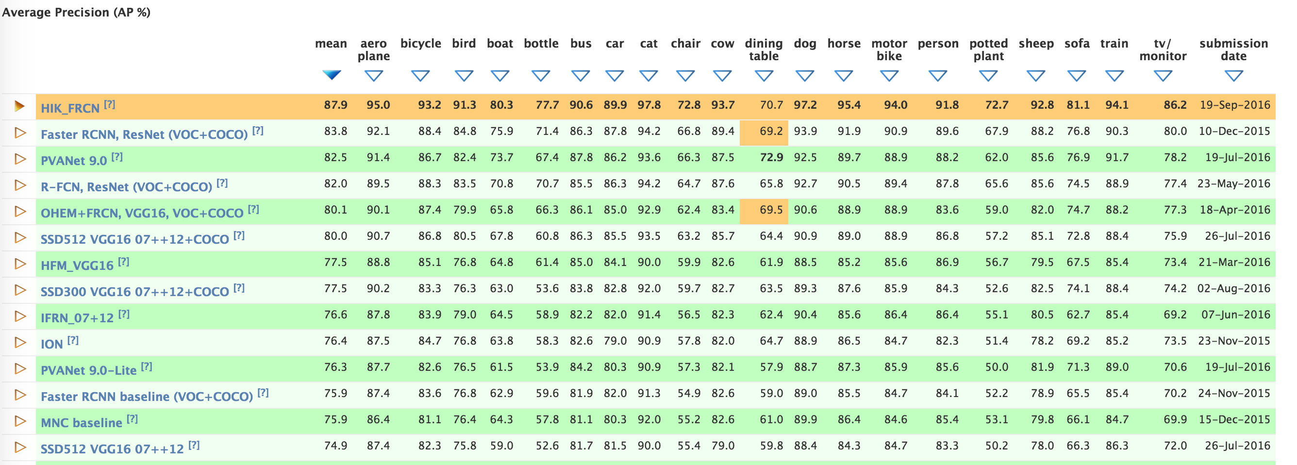
各个方法对比:http://host.robots.ox.ac.uk:8080/leaderboard/displaylb.php?cls=mean&challengeid=11&compid=4
各个方法对比:https://handong1587.github.io/deep_learning/2015/10/09/object-detection.html
代码:https://github.com/pierluigiferrari/ssd_keras/blob/master/models/keras_ssd300.py


 3384
3384

 被折叠的 条评论
为什么被折叠?
被折叠的 条评论
为什么被折叠?
 到【灌水乐园】发言


