基于K均值算法的鸢尾花聚类实验（Sklearn实现）

实验代码

##### 相关库导入部分 #####
from sklearn.datasets import load_iris
import pandas as pd
from sklearn.preprocessing import StandardScaler
from sklearn.cluster import KMeans
from sklearn.metrics import silhouette_score
import matplotlib.pyplot as plt

##### 主函数部分 #####

#### 导入鸢尾花数据集并进行格式转换 ####
# 导入sklearn自带的鸢尾花数据集
iris=load_iris()
# 将原始数据集转化为pandas的DataFrame数据表格类型，方便后续的处理过程
iris_dataset=pd.DataFrame(iris['data'],columns=iris['feature_names'])


#### 对原始数据集进行标准化预处理 ####
# 创建一个标准化处理器
# standard_transfer=StandardScaler()
# 对原始数据集进行标准化处理
# iris_dataset=pd.DataFrame(standard_transfer.fit_transform(iris_dataset))


#### 使用K均值算法（实际是K均值++算法）对鸢尾花数据进行聚类处理，通过轮廓系数确定在一定范围内的最佳聚类个数 ####
# 记录不同聚类个数情况下聚类结果的轮廓系数的列表
silhouette_scores=list()
# 记录截止到目前的最大轮廓系数
max_score=0
# 记录局部最大轮廓系数对应的聚类个数
best_clusterCount=0
# 聚类个数的变化范围是从2到10
for cluster_count in range(2,11):
    # 根据聚类个数初始化K均值聚类估计器
    Kmeans_estimator=KMeans(n_clusters=cluster_count,init="k-means++",max_iter=10000,random_state=0)
    # 用数据对K均值聚类转换器进行训练
    Kmeans_estimator.fit(iris_dataset)
    # 获取聚类模型的聚类结果
    Kmeans_result=Kmeans_estimator.predict(iris_dataset)
    # 计算轮廓系数并判断是否更新最大轮廓系数
    judge_score= silhouette_score(iris_dataset,Kmeans_result)
    # 将轮廓系数添加到列表中
    silhouette_scores.append(judge_score)
    # 判断当前轮廓系数是否为最优值，如果是则更新局部最大轮廓系数值和对应的聚类个数
    if judge_score>max_score:
        max_score=judge_score
        best_clusterCount=cluster_count
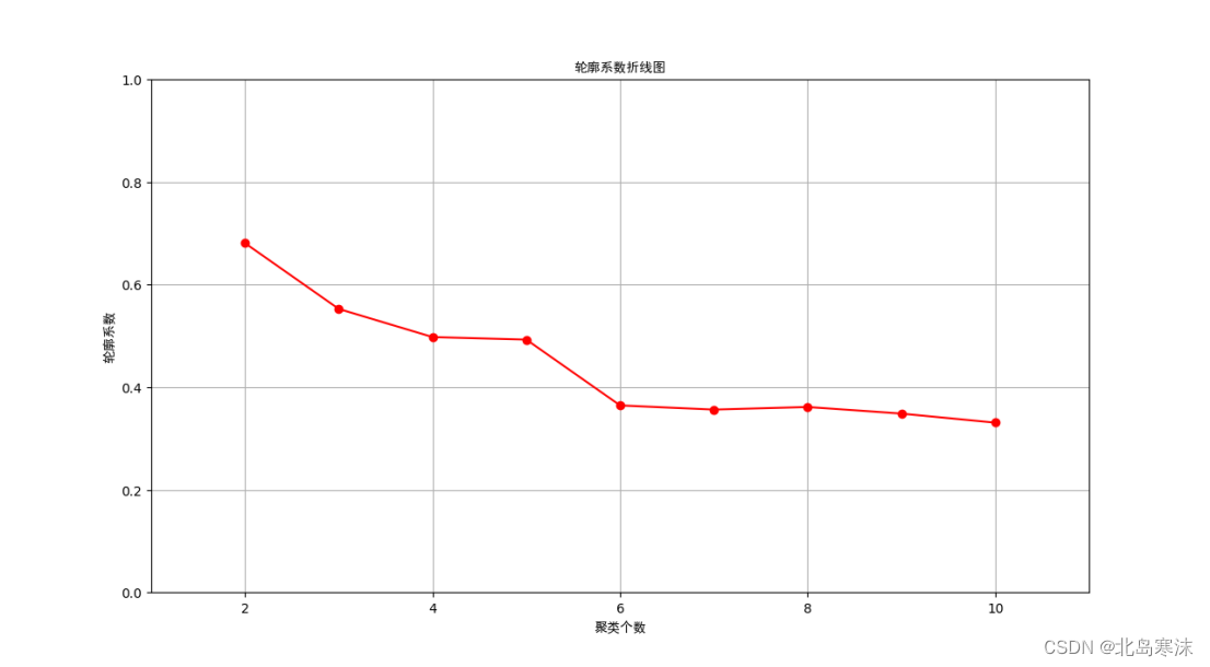
## 绘制轮廓系数折线图 ##
# 为轮廓系数折线图编号1
plt.figure(1)
plt.xlabel("聚类个数",fontproperties="Simhei")
plt.ylabel("轮廓系数",fontproperties="Simhei")
plt.axis([1,11,0,1])
plt.grid(True)
plt.title("轮廓系数折线图",fontproperties="Simhei")
plt.plot(range(2,11),silhouette_scores,'r-o')
# 展示绘制结果
plt.show()

#### 确定最优的聚类个数后，对最优聚类个数情况下的聚类结果进行绘图展示 ####
print("通过轮廓系数比较得出的最佳聚类个数是：",best_clusterCount,",对应的最大轮廓系数为：",max_score)
Kmeans_estimator=KMeans(n_clusters=best_clusterCount,init="k-means++",max_iter=10000,random_state=0)
Kmeans_estimator.fit(iris_dataset)
labels=Kmeans_estimator.labels_
Kmeans_result=Kmeans_estimator.predict(iris_dataset)

### 再原始的数据表格中添加一列，表示聚类的结果 ###
iris_dataset['cluster_result']=Kmeans_result

### 对总体样本集按照不同的聚类结果进行划分 ###
iris_dataset1 = iris_dataset[labels == 0]
iris_dataset2 = iris_dataset[labels == 1]
# iris_dataset3 = iris_dataset[labels == 2]

### 绘制聚类结果（分为四组情况进行绘制） ###

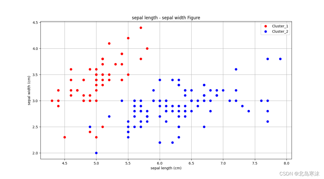
## 聚类结果展示1 ##
plt.figure(2)
plt.xlabel("sepal length (cm)")
plt.ylabel("sepal width (cm)")
plt.grid(True)
plt.title("sepal length - sepal width Figure")
line1,=plt.plot(iris_dataset1['sepal length (cm)'],iris_dataset1['sepal width (cm)'],"r o")
line2,=plt.plot(iris_dataset2['sepal length (cm)'],iris_dataset2['sepal width (cm)'],"b o")
# line3,=plt.plot(iris_dataset3['sepal length (cm)'],iris_dataset3['sepal width (cm)'],"g o")
plt.legend([line1,line2],["Cluster_1","Cluster_2"])
# plt.legend([line1,line2,line3],["Cluster_1","Cluster_2","Cluster_3"])
# 展示绘制结果
plt.show()

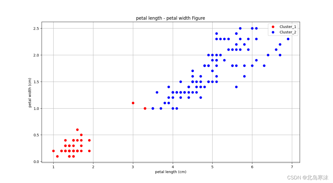
## 聚类结果展示2 ##
plt.figure(3)
plt.xlabel("petal length (cm)")
plt.ylabel("petal width (cm)")
plt.grid(True)
plt.title("petal length - petal width Figure")
line1,=plt.plot(iris_dataset1['petal length (cm)'],iris_dataset1['petal width (cm)'],"r o")
line2,=plt.plot(iris_dataset2['petal length (cm)'],iris_dataset2['petal width (cm)'],"b o")
# line3,=plt.plot(iris_dataset3['petal length (cm)'],iris_dataset3['petal width (cm)'],"g o")
plt.legend([line1,line2],["Cluster_1","Cluster_2"])
# plt.legend([line1,line2,line3],["Cluster_1","Cluster_2","Cluster_3"])
# 展示绘制结果
plt.show()

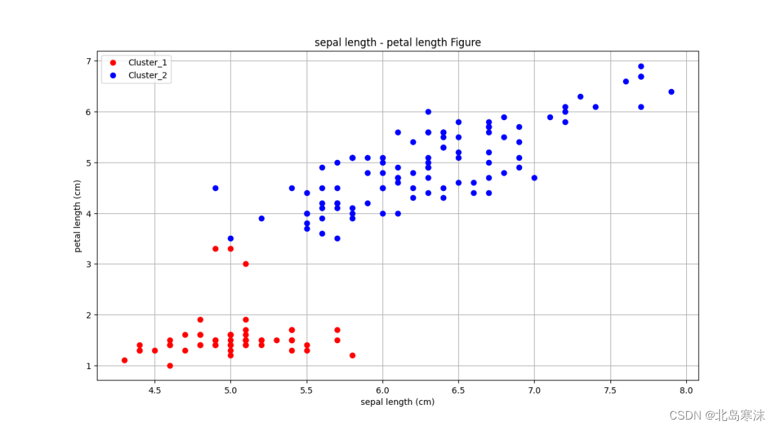
## 聚类结果展示3 ##
plt.figure(4)
plt.xlabel("sepal length (cm)")
plt.ylabel("petal length (cm)")
plt.grid(True)
plt.title("sepal length - petal length Figure")
line1,=plt.plot(iris_dataset1['sepal length (cm)'],iris_dataset1['petal length (cm)'],"r o")
line2,=plt.plot(iris_dataset2['sepal length (cm)'],iris_dataset2['petal length (cm)'],"b o")
# line3,=plt.plot(iris_dataset3['sepal length (cm)'],iris_dataset3['petal length (cm)'],"g o")
plt.legend([line1,line2],["Cluster_1","Cluster_2"])
# plt.legend([line1,line2,line3],["Cluster_1","Cluster_2","Cluster_3"])
# 展示绘制结果
plt.show()

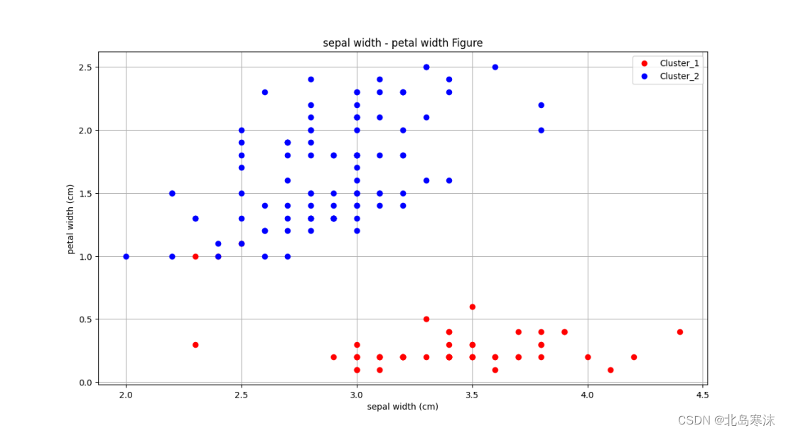
## 聚类结果展示4 ##
plt.figure(4)
plt.xlabel("sepal width (cm)")
plt.ylabel("petal width (cm)")
plt.grid(True)
plt.title("sepal width - petal width Figure")
line1,=plt.plot(iris_dataset1['sepal width (cm)'],iris_dataset1['petal width (cm)'],"r o")
line2,=plt.plot(iris_dataset2['sepal width (cm)'],iris_dataset2['petal width (cm)'],"b o")
# line3,=plt.plot(iris_dataset3['sepal width (cm)'],iris_dataset3['petal width (cm)'],"g o")
plt.legend([line1,line2],["Cluster_1","Cluster_2"])
# plt.legend([line1,line2,line3],["Cluster_1","Cluster_2","Cluster_3"])
# 展示绘制结果
plt.show()

结果展示