


逻辑回归是一种应用非常广泛的分类算法,同时也广泛地用于排序场景。如果样本集是线性可分的,逻辑回归是一个效果比较好的分类器。对于非线性特征,可以通过特征工程将其线性化。这种算法本身不具有选择重要特征的功能,通常利用l2或l1正则化方法(关于l2和l1的对比参见)做特征选择。由于逻辑回归的计算简单,具有高效性,它可以用于大数据场景,也可以利用分布式计算来加速。
下面是利用MATLAB求解带有L1正则项逻辑回归的相关代码:
非分布式版本:
function [z, history] = logreg(A, b, mu, rho, alpha)
% logreg   Solve L1 regularized logistic regression via ADMM

%

% [z, history] = logreg(A, b, mu, rho, alpha)

%

% solves the following problem via ADMM:

%

%   minimize   sum( log(1 + exp(-b_i*(a_i'w + v)) ) + m*mu*norm(w,1)

%

% where A is a feature matrix and b is a response vector. The scalar m is

% the number of examples in the matrix A.

%

% This solves the L1 regularized logistic regression problem. It uses

% a custom Newton solver for the x-step.

%

% The solution is returned in the vector x = (v,w).

%

% history is a structure that contains the objective value, the primal and

% dual residual norms, and the tolerances for the primal and dual residual

% norms at each iteration.

%

% rho is the augmented Lagrangian parameter.

%

% alpha is the over-relaxation parameter (typical values for alpha are

% between 1.0 and 1.8).

%

%

% More information can be found in the paper linked at:

% http://www.stanford.edu/~boyd/papers/distr_opt_stat_learning_admm.html

%

t_start = tic;
Global constants and defaults
QUIET    = 0;
MAX_ITER = 1000;
ABSTOL   = 1e-4;
RELTOL   = 1e-2;
Data preprocessing
[m, n] = size(A);
ADMM solver
x = zeros(n+1,1);
z = zeros(n+1,1);
u = zeros(n+1,1);

if ~QUIET
    fprintf('%3s\t%10s\t%10s\t%10s\t%10s\t%10s\n', 'iter', ...
      'r norm', 'eps pri', 's norm', 'eps dual', 'objective');
end

for k = 1:MAX_ITER    % x-update
    x = update_x(A, b, u, z, rho);    % z-update with relaxation
    zold = z;
    x_hat = alpha*x + (1-alpha)*zold;
    z = x_hat + u;
    z(2:end) = shrinkage(z(2:end), (m*mu)/rho);

    u = u + (x_hat - z); % diagnostics, reporting, termination checks
    history.objval(k)  = objective(A, b, mu, x, z);

    history.r_norm(k)  = norm(x - z);
    history.s_norm(k)  = norm(rho*(z - zold));


    history.eps_pri(k) = sqrt(n)*ABSTOL + RELTOL*max(norm(x), norm(z));
    history.eps_dual(k)= sqrt(n)*ABSTOL + RELTOL*norm(rho*u);

    if ~QUIET
        fprintf('%3d\t%10.4f\t%10.4f\t%10.4f\t%10.4f\t%10.2f\n', k, ...
            history.r_norm(k), history.eps_pri(k), ...
            history.s_norm(k), history.eps_dual(k), history.objval(k));
    end


    if history.r_norm(k) < history.eps_pri(k) && ...
       history.s_norm(k) < history.eps_dual(k)
        break;
endend

if ~QUIET
    toc(t_start);
end
end

function obj = objective(A, b, mu, x, z)
    m = size(A,1);
    obj = sum(log(1 + exp(-A*x(2:end) - b*x(1)))) + m*mu*norm(z,1);
end

function x = update_x(A, b, u, z, rho, x0)    % solve the x update
    %   minimize [ -logistic(x_i) + (rho/2)||x_i - z^k + u^k||^2 ]
    % via Newton's method; for a single subsystem only.
    alpha = 0.1;
    BETA  = 0.5;
    TOLERANCE = 1e-5;
    MAX_ITER = 50;
    [m n] = size(A);
    I = eye(n+1);
    if exist('x0', 'var')
        x = x0;    else
        x = zeros(n+1,1);
    end
    C = [-b -A];
    f = @(w) (sum(log(1 + exp(C*w))) + (rho/2)*norm(w - z + u).^2);
for iter = 1:MAX_ITER
        fx = f(x);
        g = C'*(exp(C*x)./(1 + exp(C*x))) + rho*(x - z + u);
        H = C' * diag(exp(C*x)./(1 + exp(C*x)).^2) * C + rho*I;
        dx = -H\g;   % Newton step
        dfx = g'*dx; % Newton decrement
        if abs(dfx) < TOLERANCE
break;
end
        % backtracking
        t = 1;
while f(x + t*dx) > fx + alpha*t*dfx
            t = BETA*t;
end
        x = x + t*dx;
end

end

function z = shrinkage(a, kappa)
    z = max(0, a-kappa) - max(0, -a-kappa);
end
下面是分布式实现:
function [z, history] = distr_l1_logreg(A, b, mu, N, rho, alpha)
% distr_l1_logreg   Solve distributed L1 regularized logistic regression

%

% [x, history] = distr_l1_logreg(A, b, mu, N, rho, alpha)

%

% solves the following problem via ADMM:

%

%   minimize   sum( log(1 + exp(-b_i*(a_i'w + v)) ) + m*mu*norm(w,1)

%

% where A is a feature matrix and b is a response vector. The scalar m is

% the number of examples in the matrix A.

%

% This solves the L1 regularized logistic regression problem. It uses

% a custom Newton solver for the x-step. This version solves a distributed

% version of L1 regularized logistic regression.

%

% The solution is returned in the vector x = (v,w).

%

% history is a structure that contains the objective value, the primal and

% dual residual norms, and the tolerances for the primal and dual residual

% norms at each iteration.

%

% N is the number of subsystems to use to split the examples. This code

% will (serially) solve N x-updates with m / N examples per subsystem.

% Therefore, the number of examples, m, should be divisible by N. No error

% checking is done.

%

% rho is the augmented Lagrangian parameter.

%

% alpha is the over-relaxation parameter (typical values for alpha are

% between 1.0 and 1.8).

%

% This example requires the "MATLAB Interface for L-BFGS-B" and L-BFGS-B

% installed. These can be acquiured at

% http://www.cs.ubc.ca/~pcarbo/lbfgsb-for-matlab.html.

%

%

% More information can be found in the paper linked at:

% http://www.stanford.edu/~boyd/papers/distr_opt_stat_learning_admm.html

%

t_start = tic;
Global constants and defaults
QUIET    = 0;
MAX_ITER = 1000;
ABSTOL   = 1e-4;
RELTOL   = 1e-2;
Preprocessing
[m, n] = size(A);
m = m / N;  % should be divisible
ADMM solver
x = zeros(n+1,N);
z = zeros(n+1,N);
u = zeros(n+1,N);
if ~QUIET
    fprintf('%3s\t%10s\t%10s\t%10s\t%10s\t%10s\t%10s\n', 'iter', '# bfgs', ...
      'r norm', 'eps pri', 's norm', 'eps dual', 'objective');
end

p = size(z,1);
C = [-b -A]';
global BFGS_ITERS;  % global variable to keep track of bfgs iterations

bfgs_iters = zeros(N,1);
for k = 1:MAX_ITER    % serial x-update
    for i = 1:N,
        K = C(:,1+(i-1)*m:i*m)';
        x(:,i) = bfgs_update(K, u(:,i), z(:,i), rho, N, x(:,i));
        bfgs_iters(i) = BFGS_ITERS;
    end

    % z-update with relaxation
    zold = z;
    x_hat = alpha*x + (1-alpha)*zold;
    ztilde = mean(x_hat + u,2);
    ztilde(2:end) = shrinkage( ztilde(2:end), (m*N)*mu/(rho*N) );

    z = ztilde*ones(1,N);    % u-update
    u = u + (x_hat - z);    % diagnostics, reporting, termination checks
    history.objval(k)  = objective(A, b, mu, x, z(:,1));

    history.r_norm(k)  = norm(x - z, 'fro');
    history.s_norm(k)  = norm(rho*(z - zold),'fro');

    history.LBFGS_iters(:,k) = bfgs_iters;

    history.eps_pri(k) = sqrt(p*N)*ABSTOL + RELTOL*max(norm(x,'fro'), norm(z,'fro'));
    history.eps_dual(k)= sqrt(p*N)*ABSTOL + RELTOL*norm(rho*u,'fro');
    if ~QUIET
        fprintf('%3d\t%10d\t%10.4f\t%10.4f\t%10.4f\t%10.4f\t%10.2f\n', k, sum(bfgs_iters), ...
            history.r_norm(k), history.eps_pri(k), ...
            history.s_norm(k), history.eps_dual(k), history.objval(k));
    end


    if history.r_norm(k) < history.eps_pri(k) && ...
       history.s_norm(k) < history.eps_dual(k)
        break;
    end

end

if ~QUIET
    toc(t_start);
end

z = z(:,1);
end

function obj = objective(A, b, mu, x, z)
    m = size(A,1);
    obj = sum(log(1 + exp(-A*z(2:end) -b*z(1)))) + m*mu*norm(z(2:end),1);
end

function [x t] = bfgs_update(C, u, z, rho, N, x0)    % solve the x update
    %   minimize [ -logistic(x_i) + (rho/2)||x_i - z^k + u^k||^2 ]
    % via L-BFGS

    [m n] = size(C);

    auxdata{1} = C;
    auxdata{2} = z;
    auxdata{3} = u;
    auxdata{4} = rho;

    x = lbfgsb(x0, -Inf*ones(n,1), +Inf*ones(n,1), 'l2_log', 'l2_log_grad', auxdata, 'record_bfgs_iters');
end

function z = shrinkage(a, kappa)
    z = max(0, a-kappa) - max(0, -a-kappa);
end
总结下logistic regression的优缺点。
优点:
实现简单,较多地应用于工业问题(如商品排序,商品推荐)上;
计算量比较小,速度快,所需存储资源低;
能够给出观测样本概率分数,方便排序;
可以利用L2正则化来解决多重共线性问题;
缺点:
当特征空间(样本维数)很大时,性能不是很好;
容易欠拟合,可能会导致准确度较低;
只能处理二分类问题(泛化版本softmax可用于多分类),需线性可分;
对于非线性特征,需要利用特诊工程方法进行转换,使其线性化;
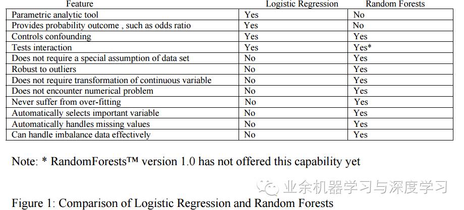
最后给出逻辑回归和随机森林的对比图,顺便预告一下下篇内容(什么内容呢,且听下回分解)
参考资料:
https://www.quora.com/What-are-the-advantages-of-different-classification-algorithms
http://d-scholarship.pitt.edu/7034/1/realfinalplus_ETD2006.pdf
代码来源:
https://web.stanford.edu/~boyd/papers/admm/logreg-l1/distr_l1_logreg.html
https://web.stanford.edu/~boyd/papers/admm/logreg-l1/logreg.html


 4258
4258


 被折叠的 条评论
为什么被折叠?
被折叠的 条评论
为什么被折叠?
 到【灌水乐园】发言


