


 本文介绍了如何在UnrealEngine5的Niagara系统中使用SimulationStage、Grid3D、PBD和SDF等技术进行高级粒子效果的创建,包括定制生命周期、纹理采样、渲染目标操作以及与外部系统交互等内容。
It is an reading note of UE5 Niagara Advanced Example, related about usage of Simulation Stage, Grid 3D, PBD, SDF and so on.
The article can’t cover all details, it just a reading note. Implementation details are so complex that it is recommended to have a look on original source.
In offical showcase project ContentExample, you can see detailed comment in Niagara System examples.
Niagara_Particles level is about basic of Niagara, here we assume readers have read it. This article mostly focus on Niagara_Advanced_Particles level.
There is also some offical tutorial:
Advanced Niagara Effects Inside Unreal
1.1 What is simulation stage
Niagara System: FIllRenderTarget.
If you need custom lifetime hook, that is my personal understanding, or in their way, stack, you should add Simulation Stage.
Enable Simulation Stages on a GPU emitter by checking “Enable Simulation Stages” in advanced emitter properties
That is weird, I can’t find Enable Simulation Stages in emitter properties, even in their example. So I leave it alone.
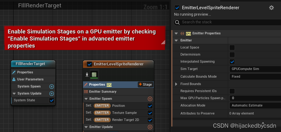
You can’t create a lifetime for arbitrary usage, UE set Simulation Stage is a For loop.
Think of a simulation stage as an additional “stack” like Particle Update. The difference is it can iterate, meaning run multiple times on a single frame across all the elements in it.Think of it like a “For Loop” in the stack.
It is also unique because its “Iteration source” can be more than just particles. A Simulation Stage can iterate over every grid cell in a Grid 2d collection to create solvers, iterate over every pixel in a render target to write to it, or iterate over every particle.
Then you know:
-
Simulation Stageis likeParticle Update, it is called per frame. -
It is a basic operation
For loop.
As for this example, you can see how it iterate all texels of render target, calc UV of render target by iteration index, sample from a texture according to this UV.
Once you know this, you will know the input and output of Simulation Stage. Input is your Niagara System parameters, and you can expose some build-in anyway. Output is void. So Simulation Stage is a function void update(user parameters).
1.2 Advect 2d Collection
Niagara System: AdvectGrid.
This example is mainly about how to sample from 2D Texture and store it into RenderTarget.
If you need some cool effect, fill RenderTarget and change sampling UV or something in Simulation Stage.
Considering adverting fluid-like emitter, I guessed it is implementing famous paper Stable Fluid at the first time. But after I click into the emitter, I found it only have two steps: diffuse and advect. These two module are completely different from what I know from Stable Fluid. Diffusion is made by simply averaging nearby four grids, advection is made by random UV offset, or in other word, random advection velocity.
How to expose variable in module to Niagara System
When I try to reproduce the work, I find my new variable created in module doesn’t appear in Niagara System Parameters window. After several tries, I find the reason that new variable must be a pin of Map get or Map set, only then it can appear in Niagara System Parameters window.
I don’t know clearly why. Maybe it is a optimation by UE, that variable which reference = 0 is auto invisible? Anyway, it confused me at first.
1.3 Communicate with External Render Targets
Niagarag System: BlurAndSetExternalRT
Variable in Niagara System can be set in external blueprint.
So now many operations on Render Texture now can be done in Niagara System.
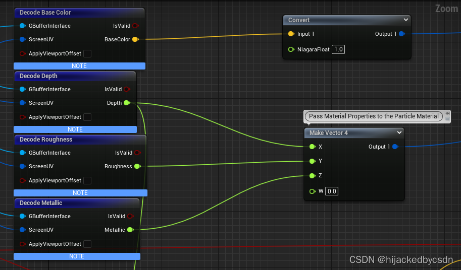
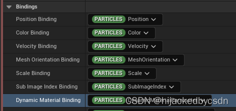
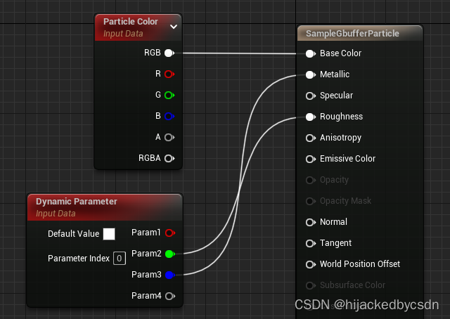
1.4 Sample GBuffer Attributes
Niagarag System: SpawnOnGBuffer
GBuffer is an input variable can be accessed.
And vector4 variables can be packed into matrix, pass into material.
More specifically saying, in the example Niagara System, vector4 depth, roughness, metallic are sampled from GBuffer access, then these vector4 variables are packed into matrix, save into DynamicMaterialParameter. In Mesh Renderer module, DynamicMaterialParameter is bind to DynamicMaterialBinding. In material, you can unpack your binding of DynamicMaterialParameter.
1.5 Skeletal Mesh Reproduction
Niagarag System: SkeletalMeshReproductionSystem_Demo_GPU
There already have module to scatter particles along given mesh UserMesh, making effect that particles seems like reconstructing UserMesh.
We find a permanent triangle coordinate for each particle. This is referenced later on to find particles’ rest positions.
Then we store some variable presistent throughout the simulation, to store the influence strength.
So during update, we can update current position of UserMesh, set it as new rest positions. And we can calculate simulation position of particles, these particle have physical nice motion.
By lerping between the simulation and the rest state we can utilize various forces without worrying about them becoming too intense. The particles will return to their rest states eventually.
1.6 Distance Field Traversal
Niagarag System: TraverseDistanceField
You can use Distance Field to get base position and motion direction on a mesh surface:
Crawl tangentially to the distance field generates a final position and velocity for each particle. It samples the distance field several times and finds the optimal position for each particle based on its geometry.
Here using Time Based State Machine to switch particles’ states.
In the example, each particle is an insect. Insect have idle state and excited state. In each iteration, for every particle, force and velocity or something in all states are calculated, so using which one is determined by solver. More specifically, there is a mask related with time to lerp the two state.
2.1 Particle Attribute Reader
Niagarag System: AttributeReaderRing
This example shows how to use Attribute Reader. I may consider it as a access of other emitter, because when initializing an Attribute Reader, you assign a name of emitter. Then in your custom module, you can access certain particle property from assigned emitter by given index.
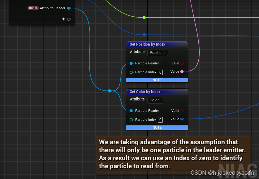
2.2 Follow The Leader 1.0
Niagarag System: AttributeReaderFollow
Similar to previous.
2.3 Spawn Particles From Another Emitter
Niagarag System: AttributeReaderStreamers
Using Spawn Particles from Other Emitter and Sample Particles from Other Emitter.
Another usage of Attribute Reader.
2.4 Iterative Constraints
Niagarag System: Chain_SimulationStages
Usage of Attribute Reader in examples above is reading other emitter, now here is an example of reading self.
What can you do if you can read self property> For example, you can query neighbor particle index i-1, i+1 close to i, then you can make a constraint like a chain.
3.1 Color Copy by Cell
Niagarag System: ColorQuery
What is Neighbor
Grid 3D have many cells, each cell logically responds to a world space.
Element in one cell are named Neighbor. It may confuse to some extent, neighbor of what? Is it neighbor particle of the cell? No, it is just element of one cell, in case of Grid 3D.
+-----------+-----------+
| neighbor1 | neighbor1 |
| neighbor2 |           |
|           |           |
+-----------+-----------+
| neighbor1 | neighbor1 |
|           | neighbor2 |
|           | neighbor3 |
+-----------+-----------+
I guess neighbor is a conventional alias, becuase UE example likes name Grid 3D as NeighborGrid. If you have a NeighborGrid, then you call element of NeighborGrid as neighbor naturally. Why call it NeighborGrid? Still guess its meaning is “Grid used to find Neighbor”, so NeighborGrid is an abbreviation to address its usage.
Transform Martix
Transform martixs have been done by UE, in module Grid 3D Create Unit to World Transform, so access grid 3d become easier.
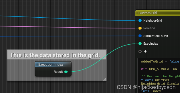
Writting to Grid 3D
This code from module Fill Neighbor Grid 3D is about writting particle index into Grid 3D:
-
transform world position into unit position,
-
map unit position into grid 3d index,
-
map grid 3d index into grid linear index,
-
access
particle indexby grid linear indexwhere writing
particle indexis usingSetParticleNeighbor, andparticle indexis namedExection indexin module built-in.Exection indexrepresent the sequence of particles are exected shading in current frame, so it will change over frame.
AddedToGrid = false;

#if GPU_SIMULATION

// Derive the Neighbor Grid Index from the world position
float3 UnitPos;
NeighborGrid.SimulationToUnit(Position, SimulationToUnit, UnitPos);

int3 Index;
NeighborGrid.UnitToIndex(UnitPos, Index.x,Index.y,Index.z);

// Verify that the derived index is valid.
int3 NumCells;
NeighborGrid.GetNumCells(NumCells.x, NumCells.y, NumCells.z);

if (Index.x >= 0 && Index.x < NumCells.x &&
    Index.y >= 0 && Index.y < NumCells.y &&
	Index.z >= 0 && Index.z < NumCells.z)
{
    int LinearIndex;
    NeighborGrid.IndexToLinear(Index.x, Index.y, Index.z, LinearIndex);

    // Increment the neighbor count for this cell. This records the number of overlaps
    // and can return a higher count than the MaxNeighborsPerCell
    int PreviousNeighborCount;
    NeighborGrid.SetParticleNeighborCount(LinearIndex, 1, PreviousNeighborCount);

    int MaxNeighborsPerCell;
    NeighborGrid.MaxNeighborsPerCell(MaxNeighborsPerCell);

    // Limit the number of neighbors added to each cell
    if (PreviousNeighborCount < MaxNeighborsPerCell)
    {
        AddedToGrid = true;

        int NeighborGridLinear;
        NeighborGrid.NeighborGridIndexToLinear(Index.x, Index.y, Index.z, PreviousNeighborCount, NeighborGridLinear);

        int IGNORE;
        NeighborGrid.SetParticleNeighbor(NeighborGridLinear, ExecIndex, IGNORE);
    }
}
#endif
One thing confused me is NeighborGrid.SetParticleNeighborCount(LinearIndex, 1, PreviousNeighborCount); contains function that increments the neighbor count, and it is hard to get an intuition about it.
Next module Find Closest Neighbor is also valuable, it tells about how to read particle index from Grid 3D.
NeighborIndex = -1;

#if GPU_SIMULATION

bool Valid;

// Derive the Neighbor Grid Index from the world position
float3 UnitPos;
NeighborGrid.SimulationToUnit(Position, SimulationToUnit, UnitPos);

int3 Index;
NeighborGrid.UnitToIndex(UnitPos, Index.x,Index.y,Index.z);

// Initialize the closest distance to a really large number
float neighbordist =  3.4e+38;

// loop over all neighbors in this cell
int MaxNeighborsPerCell;
NeighborGrid.MaxNeighborsPerCell(MaxNeighborsPerCell);

for (int i = 0; i < MaxNeighborsPerCell; ++i)
{
    // Find the ExecIndex for the current neighbor particle
    int NeighborLinearIndex;
    NeighborGrid.NeighborGridIndexToLinear(Index.x, Index.y, Index.z, i, NeighborLinearIndex);

    int CurrNeighborIdx;
    NeighborGrid.GetParticleNeighbor(NeighborLinearIndex, CurrNeighborIdx);

    // Only proceed if the returned index is valid. This is most often triggered
    // by there being fewer neighbors in the cell than the MaxNeighborsPerCell limit.
    if (CurrNeighborIdx != -1)
    {
        // Use the Attribute Reader to query the position of the neighbor particle
        float3 NeighborPos;
        AttributeReader.GetVectorByIndex<Attribute="Position">(CurrNeighborIdx, Valid, NeighborPos);

        // Compare the distance found maintaining the closest
        const float3 delta = Position - NeighborPos;
        const float dist = length(delta);

        if( dist < neighbordist )
        {
            neighbordist = dist;
            NeighborIndex = CurrNeighborIdx;
        }
    }
}

#endif
Assume that you have grid cell A, grid index of A is known, so NeighborGrid.NeighborGridIndexToLinear(Index.x, Index.y, Index.z, i, NeighborLinearIndex); gets i-th neighbor of grid cell A.
The neighbor is represented as grid linear index, so NeighborGrid.GetParticleNeighbor(NeighborLinearIndex, CurrNeighborIdx); is querying particle index Grid 3D according to this grid linear index.
Finally you get particle index CurrNeighborIdx, using Attribute Reader, you can access property of certain particle.
3.2 Dynamic Grid Transform
Niagarag System: DynamicGridTransforms
Here Initialize Neighbor Grid module is a combination of setting resolution and calcuating transform martixs.
The example is used to debug, it transform particle position by WorldToGridUnit, pass it into material, in material, if position is within 0~1, keep red, else mask by green.
3.3 Max Neighbors Per Cell
Niagarag System: PropagateNeighbors
One grid cell has maxium count of elements, if injection to grid cell is fail, it will be black, else it is white.
The reason some particle is black, is becuase if injection fails, the shading will early terminate.
So this example shows the importance of max element count of grid cell.
3.4 Color Propagation
Niagarag System: PropagateNeighbors
Usage of querying neighbor particles.
The example store PropagateValue for each particle. When blending two particles’ color, PropagateValue determine the weight. One with higher PropagateValue gets higher weight.
There is a parameter CellRadius, it determine neighbor searching radius.
3.5 Follow The Leader 2.0
Niagara System: FollowTheLeaders
Another usage of querying neighbor particles.
There is a parameter CellRadius, it determine neighbor searching radius.
After finding neighbor particles, blending the two particles’ velocity and color.
3.6 Position Based Dynamics
Niagara System: PBD
Store Exection index into Grid 3D is packed as Populate Neighbor Grid module.
PBD collision is packed into PBD Particle Collision module.
The bounce velocity is calcuate according to particle mass, collision normal, and two colliders’ Unyielding property.
3.7 Plexus
Niagara System: Plexus
PBD part is the same, this example is about how to find most fit three neighbor particles.
3.8 Structural Support
Niagara System: StructuralSupport
First emitter spawn particles following PBD, and all particles are Unyielding. It means all particle closen to each other and fixed in space.
Second emitter copy all particles position from first emitter, sort all particle, make parent-child relationship.
The connection building can refer to Plexus example, but here is more concern: parent-child references should be non-circular.
In third emitter, at the begining, all particles are Unyielding. But as time goes, all particles have chance to be yielding. When particles change to be yielding, its velocity will be calculate under gravity.
In second emitter, we establish parent-child relationship. Here we use it to make sure if parent is yielding, all its children are also yielding.
3.9 Boids
Niagara System: Boids
Force to avoid mesh surface using SDF
Force to close to center
Velocity Matching
4.1 Component Renderer
Niagara System: ComponentRendererExample
Now you can use other Niagara System as particle, or using skel mesh component as renderer.
4.2 Export Particle Data to Blueprint
Niagara System: ExportParticleData_System
Niagara System itself can store blueprint handle, and export data to blueprint.
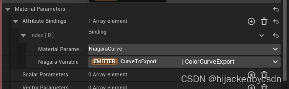
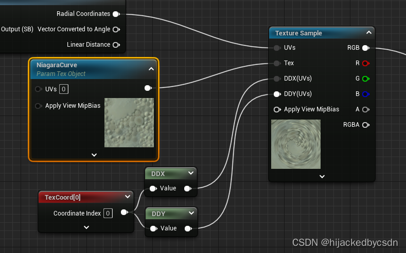
4.3 Bind Niagara Curves to Sprite Materials
Niagara System: BindCurvesToMaterials
You can create curve in Niagara System and then bind to material
4.4 Collisions in Simulation Stages
Niagara System: ParticleUpdateCollisions, SimStageCollisions
Place Collision module in Particle Update or Simulation Stage.
4.5 Dynamic Distance Fields
Niagara System: DynamicDistanceField
For each grid particles, find closet vertex among three triangle vertex.
I guess it may want to show that, each grid particle knows closet vertex, is equal to you have a distance field.
Because source of these vertex position is up to user, so it can be dynamic. For example, you can move the triangle arbitrarily.


 1816
1816

 被折叠的 条评论
为什么被折叠?
被折叠的 条评论
为什么被折叠?
 到【灌水乐园】发言


