【论文阅读】UFOMap_An_Efficient_Probabilistic_3D_Mapping_Framework_That_Embraces_the_Unknown

英文题目	UFOMap: An Efficient Probabilistic 3D Mapping Framework That Embraces the Unknown
中文名称	UFOMap:一种接纳未知的高效概率三维建图框架
发表时间	2020年3月10日
平台	IEEE Robotics and Automation Letters
作者	Daniel Duberg and Patric Jensfelt
邮箱	{ dduberg, patric}@kth.se
来源	瑞典斯德哥尔摩皇家理工学院(KTH)的机器人、感知与学习(RPL)部门
关键词	三维建图
paper && code && video	paper code video

$Abstract-3\mathrm{D}$ models are an essential part of many robotic applications. In applications where the environment is unknown a-priori, or where only a part of the environment is known, it is important that the 3D model can handle the unknown space efficiently. Path planning, exploration, and reconstruction all fall into this category.

• In this paper we present an extension to OctoMap which we call UFOMap.
• UFOMap uses an explicit representation of all three states in the map, i.e., occupied, free, and unknown. This gives, surprisingly, a more memory efficient representation.
• Furthermore, we provide methods that allow for significantly faster insertions into the octree. This enables real-time colored volumetric mapping at high resolution (below $1\mathrm{cm}$ ).
• UFOMap is contributed as a C++ library that can be used standalone but is also integrated into ROS.

$摘要-3\mathrm{D}$ 模型是许多机器人应用的重要组成部分。在环境事先未知，或仅部分环境已知的应用中，三维模型能够高效处理未知空间至关重要。路径规划、探索和重建都属于这一范畴。

• 在本文中，我们提出了对八叉树地图(OctoMap)的扩展，称之为 UFOMap。
• UFOMap 对地图中的三种状态(即占用、空闲和未知)进行显式表示。令人惊讶的是，这使得表示方式在内存使用上更加高效。
• 此外，我们提供了一些方法，能够显著加快向八叉树中插入数据的速度。这使得高分辨率(低于 $1\mathrm{cm}$)的实时彩色体素建图成为可能。
• UFOMap 以 C++ 库的形式提供，既可以独立使用，也可以集成到机器人操作系统(ROS)中。

I. INTRODUCTION

一、引言

Many robot tasks require a 3D model of the environment to be completed.

• For navigation and manipulation tasks the model is often used to calculate collision free paths
• and in exploration to determine where new information can be found and how to get to it.
• 3D SLAM updates the model and localizes the robot using it.

许多机器人任务需要一个环境的三维模型才能完成。

• 对于导航和操作任务，该模型通常用于计算无碰撞路径；
• 在探索任务中，用于确定在哪里可以找到新信息以及如何到达那里。
• 三维同时定位与地图构建(3D SLAM)会更新模型并利用它对机器人进行定位。

A number of different methods for modeling 3D environments exists: point clouds, elevation maps [1], multi-level surface maps [2], octrees [3], and signed distance fields [4]. All of these methods are able to represent occupied and free space. However, only octrees and signed distance fields are able to represent the unknown space. Moreover, point clouds, elevation maps, and multi-level surface maps are not able to represent arbitrary $3\mathrm{D}$ environments.

存在多种对三维环境进行建模的方法:点云、高程图 [1]、多级表面图 [2]、八叉树 [3] 和有符号距离场 [4]。所有这些方法都能够表示占用空间和空闲空间。

• 然而，只有八叉树和有符号距离场能够表示未知空间。
• 此外，点云、高程图和多级表面图无法表示任意 $3\mathrm{D}$ 环境。

OctoMap [5], one of the most popular mapping frameworks, is based on octrees. It provides a readily available, reliable, and efficient 3D mapping framework. OctoMap provides researchers, also those not focusing on mapping, an off the shelf solution for mapping. While OctoMap excels in many use cases, there exist certain areas where it can be improved. In this paper we focus on two areas.

八叉树地图(OctoMap)[5] 是最流行的建图框架之一，它基于八叉树。它提供了一个现成的、可靠且高效的三维建图框架。八叉树地图为研究人员(包括那些不专注于建图的研究人员)提供了一个现成的建图解决方案。虽然八叉树地图在许多用例中表现出色，但仍有一些方面可以改进。在本文中，我们关注两个方面。

First, in OctoMap, unknown space is not modeled explictly as occupied and free space. In algorithms where the unknown space is used extensively, OctoMap’s implicit representation of unknown space can be a bottleneck. Use cases where this can be a problem are, for example, collision checking, path planning where we want to know if it is possible for a robot to move from one location to another and next-best view exploration methods such as [6], [7], [8], and [9]. In the first two cases the common workaround is to treat unknown space as free space [10], [11]. This way, only occupied space has to be considered in the collision checking. However, this increases the probability of collisions. Regarding the third use case, [9] states that “computing volumetric information gains can account for up to 95% of a planner’s run-time.” The information gain for a certain sensor/robot pose in an exploration scenario is typically calculated as a function of the unknown space. In [7] the information gain is approximated, leading to a reduced need to access unknown space in the OctoMap and it is one of the major contributing factors of the performance improvement over the baseline [6].

• 首先，在八叉树地图中，未知空间不像占用空间和空闲空间那样被显式建模。在大量使用未知空间的算法中，八叉树地图对未知空间的隐式表示可能会成为瓶颈。例如，在碰撞检测、路径规划(我们想知道机器人是否可以从一个位置移动到另一个位置)以及诸如 [6]、[7]、[8] 和 [9] 等最佳视角探索方法等用例中，这可能会成为问题。
• 在前两种情况下，常见的解决方法是将未知空间视为空闲空间 [10]、[11]。这样，在碰撞检测中只需考虑占用空间。然而，这会增加碰撞的概率。
• 关于第三种用例，[9] 指出“计算体素信息增益可能占规划器运行时间的 95%”。在探索场景中，某个传感器/机器人位姿的信息增益通常是根据未知空间计算的。在 [7] 中，对信息增益进行了近似处理，从而减少了在八叉树地图中访问未知空间的需求，这也是相对于基线 [6] 性能提升的主要因素之一。

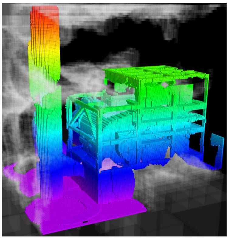
Fig. 1. UFOMap representation of an in-progress exploration of a power plant. The colored voxels are occupied space. The white voxels are unknown space which are represented explicitly in UFOMap.

图 1. 一个正在进行的发电厂探索的 UFOMap 表示。彩色体素表示占用空间。白色体素表示未知空间，在 UFOMap 中被显式表示。

Second, manipulating the content of an OctoMap is time consuming and limited. For example, inserting a single point cloud takes on the order of a second. This means that real-time volumetric mapping with an OctoMap is prohibitively slow in many applications. Furthermore, when inserting or deleting data in the map (e.g., mapping) you cannot also at the same time iterate over it to extract information (e.g. exploration). In many use cases the solution is to make a copy of the entire OctoMap structure and let consumers operate on it during the update.

• 其次，操作八叉树地图的内容既耗时又受限。例如，插入单个点云大约需要一秒钟。这意味着在许多应用中，使用八叉树地图进行实时体素建图的速度慢得令人难以接受。
• 此外，在地图中插入或删除数据(例如建图)时，不能同时对其进行遍历以提取信息(例如探索)。在许多用例中，解决方案是复制整个八叉树地图结构，并让使用者在更新期间对其进行操作。

In this paper we present an extension to OctoMap taking these shortcomings into account. The contributions of this work are as follows:

在本文中，我们考虑到这些缺点，提出了对八叉树地图的扩展。这项工作的贡献如下:

• We present a memory efficient 3D mapping framework based on octrees, called UFOMap, that explicitly represents the unknown space, together with occupied and free space.

• 我们提出了一种基于八叉树的内存高效三维建图框架，称为 UFOMap，它能够显式表示未知空间以及占用空间和空闲空间。

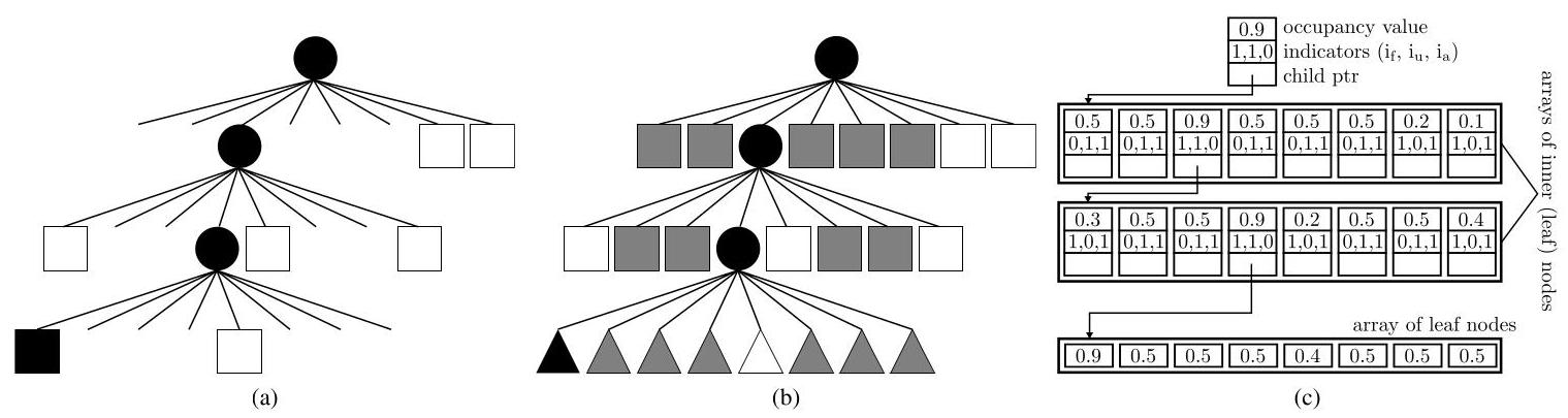
Fig. 2. Example of an octree. The OctoMap tree representation is shown in (a) and the corresponding tree representation in UFOMap is displayed in (b). Black indicates occupied space, white free space, and grey unknown space. Circles means that it is an inner node, square an inner leaf node, and triangle a leaf node. Note that OctoMap does not make a distinction between leaf nodes types. © shows how UFOMap stores that octree in memory.

图2. 八叉树示例。(a) 展示了OctoMap的树状表示，(b) 展示了UFOMap中对应的树状表示。黑色表示被占据的空间，白色表示空闲空间，灰色表示未知空间。圆形表示它是一个内部节点，正方形表示内部叶子节点，三角形表示叶子节点。请注意，OctoMap并不区分叶子节点的类型。© 展示了UFOMap如何在内存中存储该八叉树。

• We introduce different methods of incorporating data into the octree that are significantly faster than OctoMap’s. This enables real-time colored mapping at a higher resolution.

• 我们引入了将数据合并到八叉树中的不同方法，这些方法比OctoMap的方法快得多。这使得能够以更高的分辨率进行实时彩色建图。

• We improve the overall efficiency compared to OctoMap and allow for inserting/deleting data and iterate over the octree at the same time.

• 与OctoMap相比，我们提高了整体效率，并允许同时插入/删除数据和遍历八叉树。

• As opposed to OctoMap, most functions in UFOMap can work at different resolutions of the octree. Making it possible for different algorithms with varying requirements to use the same map representation.

• 与OctoMap不同，UFOMap中的大多数函数可以在八叉树的不同分辨率下工作。这使得具有不同需求的不同算法能够使用相同的地图表示。

• We validate the UFOMap mapping framework in two case studies, volumetric mapping and exploration, and compare it to OctoMap.

• 我们在两个案例研究(体积建图和探索)中验证了UFOMap建图框架，并将其与OctoMap进行了比较。

The remainder of this paper is organized as follows. Related work is presented in Section II, while in Section III the UFOMap mapping framework is presented. Implementation details are given in Section IV, followed by an evaluation of the proposed framework and case studies in Sections V and VI, respectively. Finally, Section VII summarizes and concludes the paper.

本文的其余部分组织如下。相关工作在第二节中介绍，而UFOMap建图框架在第三节中介绍。实现细节在第四节中给出，随后分别在第五节和第六节中对所提出的框架进行评估和案例研究。最后，第七节对本文进行总结和结论。

II. RELATED WORK

二、相关工作

This section gives a brief overview of different 3D map representations used in robotics.

本节简要概述了机器人技术中使用的不同三维地图表示方法。

A popular approach to model 3D environments is to dis-cretize the world into equal sized cubic volumes [12], called voxels. One of the major shortcomings of fixed grid structures is that the size of the area to be mapped has to be known a-priori. Memory requirements can also be a problem when mapping large areas at a high resolution. Voxel hashing [13] is one approach to overcome these shortcomings, where fixed sized blocks are allocated on demand.

对三维环境进行建模的一种流行方法是将世界离散化为大小相等的立方体体积 [12]，称为体素。固定网格结构的主要缺点之一是必须事先知道要映射的区域大小。在高分辨率下对大面积区域进行映射时，内存需求也可能成为问题。体素哈希 [13] 是克服这些缺点的一种方法，它根据需要分配固定大小的块。

The mapping framework Voxblox [14] uses a signed distance field [4] voxel grid, with voxel hashing for dynamic growth, as representation. It was mainly developed for planning or trajectory optimizations in the context of micro aerial vehicles (MAVs). The signed distance field representation makes trajectory optimizations faster by storing the distance to the closest obstacle in each voxel. Voxblox builds on [13] where they use a spatial hashing scheme and allocate blocks of fixed size when needed. This means that the size of the area to be mapped does not need to be known beforehand.

建图框架Voxblox [14] 使用带符号距离场 [4] 的体素网格，并采用体素哈希实现动态增长作为表示方法。它主要是为微型飞行器(MAV)的规划或轨迹优化而开发的。带符号距离场表示法通过在每个体素中存储到最近障碍物的距离，使轨迹优化更快。Voxblox基于 [13]，在其中使用空间哈希方案，并在需要时分配固定大小的块。这意味着不需要事先知道要映射的区域大小。

One of the most popular mapping frameworks is Oc-toMap [5]. OctoMap uses an octree-based data structure, as proposed in [3], to do occupancy mapping. The octree structure allows for delaying the initialization of the grid structure. It is also more memory efficient compared to Voxblox or a fixed grid structure since the information can be stored at different resolutions in the octree, without losing any precision. If the inner nodes of the octree are updated correctly, it is possible to do queries at different resolutions. This can be especially beneficial in systems where multiple algorithms are using the same map but have different computational and time requirements. These are important properties and we will therefore use an octree representation and build on OctoMap.

最流行的建图框架之一是OctoMap [5]。OctoMap使用基于八叉树的数据结构(如 [3] 中所提出的)进行占用建图。八叉树结构允许延迟网格结构的初始化。与Voxblox或固定网格结构相比，它在内存使用上也更高效，因为信息可以以不同的分辨率存储在八叉树中，而不会损失任何精度。如果八叉树的内部节点更新正确，就可以在不同的分辨率下进行查询。这在多个算法使用同一地图但具有不同计算和时间要求的系统中尤其有益。这些都是重要的特性，因此我们将使用八叉树表示并基于OctoMap进行开发。

III. UFOMAP MAPPING FRAMEWORK

三、UFOMap建图框架

This section presents the UFOMap mapping framework, which is based on OctoMap. We highlight the difference between the two frameworks to make comparison easier.

本节介绍基于OctoMap的UFOMap建图框架。我们强调这两个框架之间的差异，以便于比较。

UFOMap uses an octree data structure, just like OctoMap. An octree is a tree data structure where each node represents a cubic volume of the environment being mapped. A node can recursively be split up into eight equal sized smaller nodes, until a minimum size has been reached. The resolution of the octree is the same as the minimum node size. A visual representation of an octree can be seen in Fig. 2b.

UFOMap和OctoMap一样，使用八叉树数据结构。八叉树是一种树状数据结构，其中每个节点代表被映射环境的一个立方体体积。一个节点可以递归地拆分为八个大小相等的较小节点，直到达到最小尺寸。八叉树的分辨率与最小节点尺寸相同。八叉树的可视化表示如图2b所示。

Each node has an occupancy value indicating if the cubic volume represented by the node is occupied, free, or unknown. A probabilistic occupancy value is used in order to better handle sensor noise and dynamic environments. More specifically the log-odds occupancy value is stored in the nodes. Sensor readings can thus be fused in using only additions instead of multiplications. The log-odds occupancy value is clamped to allow for pruning the tree, as in OctoMap. Pruning can be applied when all eight of a node’s children are the same. This leads to a smaller tree, which is beneficial both in terms of memory usage and efficiency when traversing the tree.

每个节点都有一个占用值，用于指示该节点所代表的立方体体积是被占据、空闲还是未知。为了更好地处理传感器噪声和动态环境，使用了概率占用值。更具体地说，对数几率占用值存储在节点中。因此，传感器读数可以仅通过加法而不是乘法进行融合。与OctoMap一样，对数几率占用值被限制以允许对树进行剪枝。当一个节点的八个子节点都相同时，可以进行剪枝。这会使树变小，这在内存使用和遍历树的效率方面都有益。

As mentioned in Section II, the octree data structure allows for queries at different resolutions. This can speed-up applications, as well as allow for different applications that require different resolutions to share the same map. As in OctoMap, a node is defined to have the same occupancy value as the maximum occupancy value of its children. Using the maximum value is conservative and it enables doing path planning, or similar, at whichever resolution without missing any obstacles.

如第二节所述，八叉树数据结构允许以不同分辨率进行查询。这可以加速应用程序，还能让需要不同分辨率的不同应用程序共享同一地图。与OctoMap一样，一个节点被定义为具有与其子节点的最大占用值相同的占用值。使用最大值是保守的做法，它能在任何分辨率下进行路径规划或类似操作，而不会遗漏任何障碍物。

The nodes in UFOMap store three indicators, $i_f,i_u$ , and $i_a$ , which are not found in OctoMap. $i_f$ and $i_u$ indicates if a node contains free space or unknown space, respectively. No indicator is needed for the occupied space, since the occupancy value of a node is enough to tell if it contains occupied space. The third indicator, $i_a$ , indicates whether all of a node’s children are the same. $i_a$ is useful in cases were automatic pruning has been disabled, but you still want the same behaviour as if it were enabled. Automatic pruning means that the octree is automatically pruned when data is deleted or inserted into the tree. The main reason for disabling automatic pruning is for multi-threading, where you want to access and insert/delete data at the same time (see Section IV-B). It is possible to manually specify when the pruning should occur in this case. The indicators allow for increased efficiency when traversing the tree, by allowing certain branches to be ignored, for example, when only looking for unknown space.

UFOMap中的节点存储三个指标，$i_f,i_u$和$i_a$，这在OctoMap中是没有的。$i_f$和$i_u$分别表示一个节点是否包含空闲空间或未知空间。对于被占用的空间不需要指标，因为一个节点的占用值足以判断它是否包含被占用的空间。第三个指标$i_a$表示一个节点的所有子节点是否相同。$i_a$在禁用自动剪枝但仍希望具有启用自动剪枝时的相同行为的情况下很有用。自动剪枝意味着当数据被插入或删除到树中时，八叉树会自动进行剪枝。禁用自动剪枝的主要原因是为了多线程操作，在这种情况下，你希望同时访问和插入/删除数据(见第四节B)。在这种情况下，可以手动指定剪枝应该何时发生。这些指标在遍历树时可以提高效率，例如，当只寻找未知空间时，可以忽略某些分支。

The state of a node, $n$ , in OctoMap is determined by a threshold, $t_o$ :

OctoMap中一个节点的状态$n$由一个阈值$t_o$决定:

$$\mathrm{state}\left(n\right)=\{\begin{array}{ll}\text{ unknown }& \text{ if }n\text{ is null pointer }\\ \text{ occupied }& \text{ if }{t}_o\le \mathrm{occ}\left(n\right)\\ \text{ free }& \text{ else }\end{array}$$

where $\mathrm{occ}\left(n\right)$ is the occupancy value of the node $n$ . In UFOMap this has been expanded to include a threshold, $t_f$ , for when a node is free as well:

其中$\mathrm{occ}\left(n\right)$是节点$n$的占用值。在UFOMap中，这已扩展为还包括一个节点为空闲时的阈值$t_f$:

$$\mathrm{state}\left(n\right)=\{\begin{array}{ll}\text{ unknown }& \text{ if }{t}_f\le \mathrm{occ}\left(n\right)\le t_o\\ \text{ occupied }& \text{ if }{t}_o<\mathrm{occ}\left(n\right)\\ \text{ free }& \text{ if }{t}_f>\mathrm{occ}\left(n\right)\end{array}$$

these two thresholds together can be useful in certain applications. In reconstruction or exploration you want to map a certain volume. By setting $t_f=0.1$ and $t_o=0.9$ , the nodes stay in the unknown state until they have high confidence that they are either occupied or free. This can simplify the reconstruction or exploration algorithm since only unknown nodes have to be considered. In OctoMap’s case, by setting $t_o=0.9$ , a discovered node will most likely be classified as free at first. By searching for only unknown nodes in this case the map will likely end up only containing free nodes. The algorithm would therefore have to search through all the free nodes in the map, and usually there are a lot more free nodes than there are occupied nodes.

这两个阈值在某些应用中可能很有用。在重建或探索中，你希望对某个体积进行映射。通过设置$t_f=0.1$和$t_o=0.9$，节点将保持在未知状态，直到它们有很高的置信度确定它们是被占用还是空闲。这可以简化重建或探索算法，因为只需要考虑未知节点。在OctoMap的情况下，通过设置$t_o=0.9$，一个被发现的节点最初很可能被分类为空闲。在这种情况下，只搜索未知节点，地图最终可能只包含空闲节点。因此，算法必须遍历地图中的所有空闲节点，而且通常空闲节点比被占用的节点多得多。

Alternatively, if you use $t_f=0.49$ and $t_o=0.9$ , the exploration algorithm would focus its attention on the occupied space, meaning you would target higher certainty about the occupied space. This can be convenient in applications requiring reconstruction. Note that you do not have to change anything in the exploration method, and instead use these parameters to modify the exploration behaviour.

或者，如果你使用$t_f=0.49$和$t_o=0.9$，探索算法将把注意力集中在被占用的空间上，这意味着你将更关注被占用空间的更高确定性。这在需要重建的应用中可能很方便。请注意，你不必改变探索方法中的任何内容，而是使用这些参数来修改探索行为。

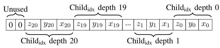
Fig. 3. Bit string representation of Morton code used in UFOMap.

图3. UFOMap中使用的莫顿码(Morton code)的位串表示。

Finally, Morton codes [15] are used to speedup traversal of the octree. To generate a Morton code, we first convert the cartesian coordinate $c=\left(c_x,c_y,c_z\right)\in {\mathbb{R}}^3$ to the octree node index tuple $k=\left(k_x,k_y,k_z\right)\in {\mathbb{N}}_0^3$ that $c$ falls into:

最后，使用莫顿码[15]来加速八叉树的遍历。为了生成莫顿码，我们首先将笛卡尔坐标$c=\left(c_x,c_y,c_z\right)\in {\mathbb{R}}^3$转换为$c$所在的八叉树节点索引元组$k=\left(k_x,k_y,k_z\right)\in {\mathbb{N}}_0^3$:

$$k_j=\lfloor \frac{c_j}{\mathrm{res}}\rfloor +2^{d_{\max }-1}\text{\hspace{1em}(1)}$$

where $d_{\max }$ is the depth of the octree. By interleaving the bits representing $k_j$ as shown in Fig. 3, the Morton code $m$ is created for $c$ . From the root node it is then possible to traverse down to the node by simply looking at the three bits of $m$ that correspond to the depth of the child and moving to that child.

其中$d_{\max }$是八叉树的深度。如图3所示，通过交错表示$k_j$的位，为$c$创建莫顿码$m$。然后从根节点开始，只需查看$m$中对应子节点深度的三位，就可以向下遍历到该子节点。

The Morton code generation has been accelerated by using integer dilation and contraction [16].

通过使用整数膨胀和收缩[16]加速了莫顿码的生成。

IV. IMPLEMENTATION DETAILS

四、实现细节

This section covers implementation details and highlights differences compared to OctoMap.

本节涵盖实现细节，并突出与OctoMap相比的差异。

A. Nodes

A. 节点

UFOMap has three different types of nodes; inner nodes, inner leaf nodes, and leaf nodes. In contrast, OctoMap has only what corresponds to the inner nodes and inner leaf nodes.

UFOMap有三种不同类型的节点:内部节点、内部叶节点和叶节点。相比之下，OctoMap只有对应于内部节点和内部叶节点的节点。

1. Inner nodes: The inner nodes are all the nodes that have children. An inner node contains a 4-byte log-odds occupancy value and an 8-byte pointer to an array of its children. In UFOMap the children are stored directly in the array, instead of the array holding pointers to the children like in OctoMap. Meaning that 64 bytes are saved for an inner node with 8 children in UFOMap compared to OctoMap. However, this also means that a node in UFOMap either must have no children or 8 children.

2. 内部节点:内部节点是所有有子节点的节点。一个内部节点包含一个4字节的对数几率占用值(log-odds occupancy value)和一个指向其子节点数组的8字节指针。在UFOMap中，子节点直接存储在数组中，而不像OctoMap那样数组保存指向子节点的指针。这意味着与OctoMap相比，在UFOMap中一个有8个子节点的内部节点可节省64字节。然而，这也意味着UFOMap中的一个节点要么没有子节点，要么有8个子节点。

The inner nodes also contain the three indicators mentioned in Section III, taking a total of 4 bytes. On a 64-bit operating system this means that the inner nodes require 16 bytes, compared to 72 bytes for OctoMap.

内部节点还包含第三节中提到的三个指示符，总共占用4字节。在64位操作系统上，这意味着内部节点需要16字节，而OctoMap需要72字节。

2. Inner leaf nodes: Inner leaf nodes are exactly the same as the inner nodes, described in Section IV-A1. The only distinction is that the inner leaf nodes have no children, meaning the child pointer is a null pointer. Once an inner leaf node gets a child it is considered an inner node. In OctoMap this is the only kind of leaf node that exist.

3. 内部叶节点:内部叶节点与第四节A1中描述的内部节点完全相同。唯一的区别是内部叶节点没有子节点，即子节点指针为空指针。一旦一个内部叶节点有了子节点，它就被视为内部节点。在OctoMap中，这是唯一存在的叶节点类型。

On a 64-bit operating system an inner leaf node in UFOMap takes up 16 bytes, the same as in OctoMap.

在64位操作系统上，UFOMap中的一个内部叶节点占用16字节，与OctoMap相同。

3. Leaf nodes: The leaf nodes are more simplistic. Only the 4-byte log-odds occupancy value is stored. Compared to an inner leaf node, it is not possible for a leaf node to have children. In OctoMap the corresponding node is the inner leaf node, which takes up 16 bytes.

4. 叶节点:叶节点更简单。只存储4字节的对数几率占用值。与内部叶节点相比，叶节点不可能有子节点。在OctoMap中，对应的节点是内部叶节点，占用16字节。

The three kinds of nodes can be seen in Fig. 2c. The nodes which have an occupancy value, indicators, and a child pointer are inner nodes, and where the child pointer is empty is an inner leaf node. The nodes with only an occupancy value are the leaf nodes.

这三种节点可以在图2c中看到。具有占用值、指示符和子节点指针的节点是内部节点，子节点指针为空的是内部叶节点。只有占用值的节点是叶节点。

As stated in [5], and also seen in Table I, 80-85% of the octree nodes are (inner) leaf nodes in OctoMap. However, since OctoMap does not differentiate between inner leaf nodes and leaf nodes we see that this value drops to 71-81% in UFOMap, where the distinction is made and only leaf nodes are shown. This means that the majority of the nodes in the tree are leaf nodes. Therefore, having the dedicated leaf node data structures and by storing the children of an inner node directly in an array in UFOMap significantly reduces the memory usage over OctoMap by a factor of 3 , even though the total amount of nodes in the tree increases (see Table I).

如文献[5]所述，从表I中也可以看出，在OctoMap中，80 - 85%的八叉树节点是(内部)叶节点。然而，由于OctoMap不区分内部叶节点和叶节点，我们发现这个值在UFOMap中降至71 - 81%，在UFOMap中进行了区分，只显示叶节点。这意味着树中的大多数节点是叶节点。因此，即使树中的节点总数增加(见表I)，通过在UFOMap中使用专用的叶节点数据结构并将内部节点的子节点直接存储在数组中，与OctoMap相比，内存使用量显著减少了三分之一。

B. Multi-threading

B. 多线程

Multi-core processors are the norm in most segments nowadays. To fully utilize these processors the third indicator $i_a$ , mentioned in Section III, which indicates whether all of an inner node’s children are the same, was introduced.

如今，多核处理器在大多数领域已成为标准配置。为了充分利用这些处理器，引入了第三节中提到的第三个指示符 $i_a$，它用于指示一个内部节点的所有子节点是否相同。

When inserting data into UFOMap and OctoMap the tree is automatically pruned when possible. If pruning occurs in a thread at the same time as another thread is iterating through the tree, it can remove nodes that the iterator is currently pointing to. Making the iterator invalid, with undefined behavior if dereferenced.

当向UFOMap和OctoMap中插入数据时，树会在可能的情况下自动进行剪枝。如果在一个线程进行剪枝的同时，另一个线程正在遍历树，剪枝操作可能会移除迭代器当前指向的节点。这会使迭代器失效，如果对其进行解引用，会导致未定义行为。

To prevent this, UFOMap allows for disabling the automatic pruning. In this case $i_a$ will be used to determine if a node is an inner node or an inner leaf node. If it is the latter, it will not traverse further down the tree. This allows for inserting data and traversing the tree at the same time, while still utilizing the octree structure. It is possible to manually tell UFOMap when to prune the tree, such that the memory consumption still can remain low while maintaining thread safety.

为了防止这种情况发生，UFOMap允许禁用自动剪枝。在这种情况下，将使用 $i_a$ 来确定一个节点是内部节点还是内部叶节点。如果是后者，将不再进一步遍历树。这允许在插入数据的同时遍历树，同时仍然利用八叉树结构。可以手动告知UFOMap何时对树进行剪枝，这样在保持线程安全的同时，仍能使内存消耗保持在较低水平。

C. Integrating Point Cloud Sensor Measurements

C. 整合点云传感器测量数据

Ray tracing is used to integrate point cloud sensor measurements. When integrating a point cloud it is important that points that should be occupied gets occupied and that all points between the sensor origin and each point of the point cloud gets freed. In UFOMap there are four methods for this, each faster than the previous but with less accurate results:

使用射线追踪来整合点云传感器测量数据。在整合点云时，重要的是应被占用的点要被标记为占用，并且传感器原点与点云中每个点之间的所有点都要被标记为空闲。在UFOMap中有四种方法可以实现这一点，每种方法都比前一种更快，但结果的准确性较低:

1. Simple integrator: For each point in the point cloud we trace a ray, using [17], and free all nodes from origin to the point. We set the node in which the point lies to occupied. Same as in OctoMap.

2. 简单积分器:对于点云中的每个点，我们使用文献[17]中的方法进行射线追踪，并将从原点到该点的所有节点标记为空闲。我们将该点所在的节点标记为占用。这与OctoMap中的方法相同。

3. Discrete integrator: We use the fact that a number of points in the point cloud fall inside the same node. So by discretizing the point cloud first, the ray tracing is only done once for each node the points fall into. The ray tracing is performed towards the center of the node which means the result can be different compared to the simple integration. However, this is significantly faster for large point clouds with many points falling into the same node. The same method exists in OctoMap.

4. 离散积分器:我们利用点云中的多个点落在同一个节点内这一事实。因此，首先对点云进行离散化，对于点落入的每个节点，只进行一次射线追踪。射线追踪是朝着节点的中心进行的，这意味着与简单积分方法相比，结果可能会有所不同。然而，对于有许多点落入同一节点的大型点云，这种方法要快得多。OctoMap中也有相同的方法。

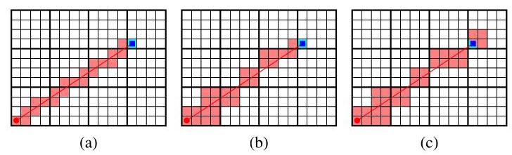
Fig. 4. Comparison of the integrators mentioned in Section IV-C, for a single ray starting at the bottom left corner (red circle) and ending near the top right corner (blue square). The red line is the line being traced. The red and blue cell(s) will be marked free or occupied by the integrator, respectively. (a) Simple/discrete integrator (b) Fast discrete integrator with $d=1$ and $n=2$ © Fast discrete integrator with $d=1$ and $n=0$ . Note that the end point will be marked both as free and occupied.

图4. 对第四节C部分中提到的积分器进行比较，针对从左下角(红色圆圈)起始并在右上角附近结束(蓝色方块)的单条射线。红色线条为正在追踪的线。红色和蓝色的单元格将分别被积分器标记为空闲或被占用。(a) 简单/离散积分器 (b) 带有 $d=1$ 和 $n=2$ 的快速离散积分器 © 带有 $d=1$ 和 $n=0$ 的快速离散积分器。请注意，终点将同时被标记为空闲和被占用。

3. Fast discrete integrator: In the fast discrete integrator, the ray tracing and discretization is performed at multiple different depths. First, a ray tracing algorithm (Eq. 2), cruder than [17], is applied at a coarser resolution, corresponding to depth $d$ . Ray tracing is done until $n$ nodes, at that resolution, away from the end node. From that node we perform a new ray tracing at lower depth until we reach depth 0 (leaf node depth) where we perform the same ray tracing as in the discrete integration. This ensures that we do not clear space behind the occupied space. The parameters $n$ and $d$ allow us to trade speed against accuracy.

4. 快速离散积分器:在快速离散积分器中，射线追踪和离散化在多个不同深度进行。首先，应用一种比文献[17]中更粗糙的射线追踪算法(公式2)，以较粗的分辨率进行，对应深度 $d$。射线追踪一直进行到距离终点节点在该分辨率下 $n$ 个节点的位置。从该节点开始，我们在较低深度进行新的射线追踪，直到达到深度0(叶节点深度)，在该深度我们执行与离散积分中相同的射线追踪。这确保我们不会清除被占用空间后面的空间。参数 $n$ 和 $d$ 使我们能够在速度和精度之间进行权衡。

$${\text{free}}_i=\text{origin}+i\cdot {\text{res}}_d\cdot \frac{\left(\text{end}-\text{origin}\right)}{\parallel \text{end}-\text{origin}\parallel }\text{,}\text{\hspace{1em}(2)}$$

$$\forall i\in 0,\dots ,\frac{\parallel \text{ end }-\text{ origin }\parallel }{{\mathrm{res}}_d}-n$$

where ${\mathrm{res}}_d$ is the resolution at the depth $d$ . The special case $d=0$ corresponds to the discrete integrator above and in the case $n=0$ space is cleared only at depth $d$ .

其中 ${\mathrm{res}}_d$ 是深度 $d$ 处的分辨率。特殊情况 $d=0$ 对应于上述离散积分器，而在情况 $n=0$ 下，仅在深度 $d$ 处清除空间。

Extra care has to be taken when inserting data into the octree at a different depth, as in the fast discrete integrator method. When clearing free space at depth $d$ we check if the node at that depth is not occupied. If it is not occupied, we can simply update the occupancy value of that node, and remove its children. If it is occupied, we will instead go down one more depth level and perform the same check until we are at a leaf node.

当像在快速离散积分器方法中那样在不同深度将数据插入八叉树时，必须格外小心。当在深度 $d$ 处清除空闲空间时，我们检查该深度的节点是否未被占用。如果未被占用，我们可以简单地更新该节点的占用值，并移除其子节点。如果被占用，我们将再向下深入一个深度级别并执行相同的检查，直到到达叶节点。

The occupied nodes are updated at the highest resolution in all three integrators. Thus, the occupied space will look mostly the same for all three methods, which is the most important aspect in most applications.

在所有三种积分器中，被占用的节点都以最高分辨率进行更新。因此，对于所有三种方法，被占用的空间看起来大致相同，这在大多数应用中是最重要的方面。

A comparison of the integrators can be seen in Fig. 4.

积分器的比较如图4所示。

D. Bounding Box

D. 边界框

UFOMap and OctoMap supports defining a bounding box to speedup operations. Only a subset of the octree has to be searched and updated. When inserting data into OctoMap only rays that begin and end inside the bounding box are integrated into the map. This can be a problem for exploration algorithms which rely on free space being cleared. In UFOMap, this problem is fixed, by moving the beginning and ending of the rays towards each other until they both are inside the bounding box.

UFOMap和OctoMap支持定义边界框以加速操作。只需搜索和更新八叉树的一个子集。当将数据插入OctoMap时，只有起点和终点都在边界框内的射线才会被整合到地图中。这对于依赖清除空闲空间的探索算法来说可能是个问题。在UFOMap中，通过将射线的起点和终点相互靠近，直到它们都在边界框内，解决了这个问题。

TABLE I

Memory consumption and number of nodes comparison between UFOMap and Octomap on the Octomar 3D scan dataset.

在Octomar 3D扫描数据集上，UFOMap和Octomap之间的内存消耗和节点数量比较。

Dataset	Memory usage			Number of nodes
	UFOMap (MB)	OctoMap (MB)	Reduction (%)	UFOMap	OctoMap	UFOMap leaves (%)	OctoMap leaves (%)
FR-078 tidyup	7.42	21.49	65.47	1642113	1369 165	80.51	85.01
FR-079 corridor	19.70	51.86	62.01	2823713	1829134	75.20	80.70
Freiburg campus	58.71	155.46	62.23	8402 193	5515178	75.10	80.96
freiburg1_360	15.98	42.05	62.00	2161849	1547112	71.72	82.53
New College	29.41	75.40	60.99	4157217	2633701	74.37	80.27

E. Accessing Data

E. 数据访问

To access the data in UFOMap, iterators are used. They are fast and they can be used to specify bounding boxes, bounding spheres and bounding frustums. Only bounding boxes are available in OctoMap. Iterators can also specify the type of nodes that should be returned, e.g., only leaves, occupied, free, unknown, contains occupied/free/unknown, or a combination of them. In comparison, OctoMap always returns free and occupied nodes. It is not possible to get the unknown nodes, and it is not possible to get only occupied nodes or only free nodes.

为了访问UFOMap中的数据，使用迭代器。它们速度快，并且可用于指定边界框、边界球和边界锥台。OctoMap中仅提供边界框。迭代器还可以指定应返回的节点类型，例如，仅叶节点、被占用节点、空闲节点、未知节点、包含被占用/空闲/未知节点，或它们的组合。相比之下，OctoMap总是返回空闲和被占用的节点。无法获取未知节点，也无法仅获取被占用节点或仅空闲节点。

F. Availability

F. 可用性

UFOMap is available as a self-contained $\mathrm{C}++$ library at https://github.com/danielduberg/UFOMap.Packages for integration with the Robot Operation System (ROS) [18] are also available. There are functions for reading and writing Oc-toMap files and converting between UFOMap and OctoMap. This facilitates the transition from OctoMap to UFOMap in an already existing system, and allows to utilize both mapping frameworks for different parts of the same system.

UFOMap作为一个自包含的 $\mathrm{C}++$ 库可在https://github.com/danielduberg/UFOMap获取。也提供了用于与机器人操作系统(ROS)[18]集成的软件包。有用于读写OctoMap文件以及在UFOMap和OctoMap之间进行转换的函数。这便于在现有系统中从OctoMap过渡到UFOMap，并允许在同一系统的不同部分使用这两种映射框架。

V. EVALUATION

V. 评估

We compare our proposed mapping framework, UFOMap, against OctoMap when it comes to memory consumption, insertion time, and in three different use cases.

我们在内存消耗、插入时间以及三种不同用例方面，将我们提出的映射框架UFOMap与OctoMap进行比较。

A. Memory Consumption and Node Count

A. 内存消耗和节点数量

In the first experiment, we compare the memory consumption between UFOMap and OctoMap on the OctoMap 3D scan dataset ${}^1$ . We analyze the memory usage when the tree has been pruned. Table I shows that UFOMap is around $38\%$ of the size of OctoMap, even though UFOMap contains more nodes in total, as seen in the same table. The increase in the number of nodes is a result of the unknown space being explicitly represented, meaning an inner node must have either 0 or 8 children. The decrease in memory usage is because of i) the smaller data structures for the leaf nodes mentioned in Section IV-A and ii) storing the child nodes directly in the child array of the inner nodes, instead of storing pointers to the children as in OctoMap.

在第一个实验中，我们在OctoMap 3D扫描数据集 ${}^1$ 上比较了UFOMap和OctoMap的内存消耗。我们分析了树被剪枝后的内存使用情况。表I显示，即使从同一表中可以看出，UFOMap的节点总数更多，但它的大小约为OctoMap的 $38\%$。节点数量的增加是由于显式表示了未知空间，这意味着内部节点必须有0个或8个子节点。内存使用量的减少是因为:i) 如第四节A所述，叶节点的数据结构更小；ii) 与OctoMap不同，UFOMap将子节点直接存储在内部节点的子数组中，而不是存储子节点的指针。

TABLE II

INSERTION TIMINGS COMPARISON BETWEEN UFOMAP AND OCTOMAP, ON THE COW DATASET ${}^2$ , WITH DIFFERENT VOXEL SIZES.

在奶牛数据集 ${}^2$ 上，不同体素大小下，UFOMap和OctoMap的插入时间比较。

Method	Voxel size (cm)	Total (ms)	Ray tracing (ms)	Insertion (ms)
UFOMap	16	${4.98} \pm {1.30}$	${4.64} \pm {1.08}$	${0.34} \pm {0.27}$
OctoMap		${5.52} \pm {1.66}$	${4.86} \pm {1.18}$	${0.66} \pm {0.56}$
UFOMap	8	${12.3} \pm {7.4}$	${10.4} \pm {5.8}$	${1.9} \pm {1.6}$
OctoMap		${16.3} \pm {10.4}$	${12.2} \pm {6.9}$	${4.1} \pm {3.7}$
UFOMap*		${8.1} \pm {3.4}$	${6.7} \pm {2.3}$	${1.4} \pm {1.1}$
${\mathrm{{UFOMap}}}^{ \dagger }$		${6.5} \pm {2.2}$	${6.0} \pm {1.8}$	${0.5} \pm {0.4}$
UFOMap	4	${60.9} \pm {44.7}$	${46.8} \pm {32.7}$	${14.1} \pm {12.2}$
OctoMap		${104.6} \pm {82.2}$	${71.8} \pm {53.0}$	${32.9} \pm {30.1}$
UFOMap*		${21.1} \pm {12.0}$	${14.3} \pm {6.7}$	${6.8} \pm {5.4}$
${\mathrm{{UFOMap}}}^{ \dagger }$		${10.9} \pm {4.7}$	${9.3} \pm {3.5}$	${1.6} \pm {1.3}$
UFOMap	2	${371} \pm {254}$	${264} \pm {176}$	${107} \pm {79}$
OctoMap		${745} \pm {548}$	${521} \pm {369}$	${224} \pm {188}$
UFOMap*		74±44	${42} \pm {22}$	${32} \pm {22}$
${\mathrm{{UFOMap}}}^{ \dagger }$		${28} \pm {15}$	20±9	9±7

B. Insertion

B. 插入

Point cloud integration time comparison between UFOMap and OctoMap is shown in Table II, using the cow dataset ${}^2$ . For both UFOMap and OctoMap the discrete integrator, mentioned in Section IV-C2, is used. UFOMap* uses the fast discrete integrator, mentioned in Section IV-C3, with $n=2$ and $d$ corresponding to the depth of the voxels at $16\mathrm{cm}$ voxel size. ${\text{UFOMap}}^{†}$ uses the fast integrator with $n=0$ and again $d$ corresponding to the depth of the voxels at $16\mathrm{cm}$ voxel size.

表II展示了在奶牛数据集 ${}^2$ 上，UFOMap和OctoMap的点云集成时间比较。对于UFOMap和OctoMap，都使用了第四节C2中提到的离散积分器。UFOMap*使用了第四节C3中提到的快速离散积分器，其中 $n=2$ 和 $d$ 对应于体素大小为 $16\mathrm{cm}$ 时体素的深度。${\text{UFOMap}}^{†}$ 使用了快速积分器，其中 $n=0$ 且 $d$ 同样对应于体素大小为 $16\mathrm{cm}$ 时体素的深度。

The total time represents the average time for a single point cloud to be integrated. Ray tracing shows the average time per point cloud for doing the ray tracing part of the insertion. Insertion shows the average time per point cloud for integrating the points calculated from the ray tracing step into the octree. The standard deviation is included for all.

总时间表示单个点云集成的平均时间。射线追踪显示了每个点云进行插入操作中射线追踪部分的平均时间。插入显示了每个点云将射线追踪步骤计算出的点集成到八叉树中的平均时间。所有数据都包含了标准差。

When only looking at the discrete integrator for UFOMap, we see that it is about two times faster at the insertion part of the integration compared to OctoMap. The ray tracing is between 1 to 2 times faster in UFOMap, which is, most likely, due to different implementation factors since both utilize the same algorithm. As the voxel size decreases, the difference between the two framework increases, in favour of UFOMap. At a voxel size of $4\mathrm{cm}$ and below, the need for the faster integrators becomes very apparent.

仅看UFOMap的离散积分器时，我们发现它在集成的插入部分比OctoMap快约两倍。UFOMap的射线追踪速度比OctoMap快1到2倍，这很可能是由于不同的实现因素，因为两者使用的是相同的算法。随着体素大小的减小，两个框架之间的差异增大，更有利于UFOMap。当体素大小为 $4\mathrm{cm}$ 及以下时，对更快积分器的需求变得非常明显。

---

${}^1$ http://ais.informatik.uni-freiburg.de/projects/datasets/octomap

${}^1$ http://ais.informatik.uni-freiburg.de/projects/datasets/octomap

---

TABLE III

COMPARISON OF TIME TAKEN TO DO COLLISION CHECKING IN UFOMAP COMPARED TO OCTOMAP.

UFOMap与OctoMap进行碰撞检查所需时间的比较。

Dataset	Voxel size (cm)	UFOMap (us/pose)	OctoMap (μs/pose)	UFOMapocto (us/pose)
FR-078 tidyup	5	2.7	23.1	14.5
FR-079 corridor	5	3.0	15.7	10.4
Freiburg campus	20	2.4	1.4	0.8
freiburg1_360	2	3.1	163.3	121.8
New College	20	2.5	1.4	0.8

UFOMap* and UFOMap ${}^{†}$ provides just that, fast integration while still clearing free space. With ${\mathrm{UFOMap}}^{†}$ scaling a lot better with the resolution and being 26 times faster than OctoMap at $2\mathrm{cm}$ voxel size.

UFOMap*和UFOMap ${}^{†}$ 正好提供了这样的功能，即在清理自由空间的同时实现快速集成。${\mathrm{UFOMap}}^{†}$ 在分辨率方面的扩展性更好，在体素大小为 $2\mathrm{cm}$ 时比OctoMap快26倍。

C. Collision Checking

C. 碰撞检查

In the first of the use cases we check if the robot, or a part of the robot, can be at a certain position in the map. That is, we check if a region of the map is free, meaning there is no occupied or unknown space in that region. This is an operation that is heavily used in sampling-based motion planners, such as RRTs. By not allowing any unknown space in this region we are more conservative and safe. We sampled 1000000 poses where at least the center of the pose was in free space. A radius of $25\mathrm{cm}$ was used. On average around $50\%$ of the poses sampled were in collision. The results are presented in Table III. We can see that UFOMap allows for faster collision checking than OctoMap in all cases but the ones with large voxels. This is most likely because of the overhead for constructing the iterators in UFOMap in these cases. The last column shows the result when using the same way to traverse the octree for collisions as in OctoMap in UFOMap. We see that this is faster than OctoMap for all resolutions. However, it is significantly slower than the default method in UFOMap, which exploits the octree structure, for the higher resolutions.

在第一个用例中，我们检查机器人或机器人的一部分是否可以处于地图中的某个特定位置。也就是说，我们检查地图的某个区域是否为空，即该区域没有被占用或未知的空间。这是基于采样的运动规划器(如RRTs)中大量使用的操作。通过不允许该区域存在任何未知空间，我们更加保守和安全。我们采样了1000000个位姿，其中至少位姿的中心位于自由空间。使用了半径为 $25\mathrm{cm}$。平均而言，采样的位姿中约有 $50\%$ 发生了碰撞。结果如表III所示。我们可以看到，除了体素较大的情况外，在所有情况下UFOMap的碰撞检查速度都比OctoMap快。这很可能是因为在这些情况下，UFOMap构建迭代器的开销较大。最后一列显示了在UFOMap中使用与OctoMap相同的方式遍历八叉树进行碰撞检查的结果。我们发现，对于所有分辨率，这种方法都比OctoMap快。然而，对于较高的分辨率，它比UFOMap中利用八叉树结构的默认方法要慢得多。

The reason for UFOMap seemingly being invariant to the voxel size can be because of the indicators $i_f$ and $i_u$ , presented in Section III, together with the iterators mentioned in Section IV-E. By specifying the bounding box and that only occupied and unknown voxels should be retrieved, UFOMap can move straight down the octree to a node that is either occupied or unknown inside the radius.

UFOMap看似与体素大小无关的原因可能在于第三节中介绍的指标 $i_f$ 和 $i_u$ ，以及第四节E部分提到的迭代器。通过指定边界框并要求仅检索被占用和未知的体素，UFOMap可以直接在八叉树中向下移动到半径内被占用或未知的节点。

For comparison reasons we have also included the time taken if only checking a region for occupied space. This corresponds to a simplification often made in collision checking to speed up the computations. The results are presented in Table IV. We can see that UFOMap is faster than OctoMap at all resolutions. Reasons for this can be the use of Morton codes for traversing the octree, perhaps less cache misses since less memory is used, or the inclusion of the indicators. Both UFOMap and OctoMap exploit the octree structure in this experiment. Hence, there is no need for UFOMap ${}^{\text{octo }}$ .

出于比较的目的，我们还记录了仅检查区域内被占用空间所需的时间。这对应于碰撞检查中为加快计算速度而常做的简化操作。结果见表四。我们可以看到，在所有分辨率下，UFOMap都比OctoMap更快。其原因可能是使用了莫顿码(Morton codes)来遍历八叉树，可能由于使用的内存较少而减少了缓存未命中的情况，或者是因为包含了这些指标。在这个实验中，UFOMap和OctoMap都利用了八叉树结构。因此，不需要UFOMap ${}^{\text{octo }}$ 。

TABLE IV

SAME AS TABLE III EXCEPT THAT THE COLLISION CHECKING IS ONLY DONE W.R.T. OCCUPIED SPACE.

与表三相同，只是碰撞检查仅针对被占用空间进行。

Dataset	Voxel size (cm)	UFOMap (us/pose)	OctoMap (μs/pose)
FR-078 tidyup	5	1.6	2.3
FR-079 corridor	5	2.1	3.6
Freiburg campus	20	1.4	1.6
freiburg1_360	2	2.2	5.3
New College	20	1.4	1.5

D. Collision Checking Along a Line Segment

D. 沿线段进行碰撞检查

In the second use case we perform collision checking along a line. For simple RRT path planning, the operations described in Sections V-C and V-D are combined.

在第二个用例中，我们沿一条线进行碰撞检查。对于简单的快速探索随机树(RRT)路径规划，将第五节C和第五节D中描述的操作结合起来。

As in Section V-C, we are conservative and require that there is no occupied or unknown space along the line. The line is defined by two randomly sampled points. As seen in Table V UFOMap is between 2 to 15 times faster than OctoMap.

与第五节C部分一样，我们采取保守策略，要求沿线没有被占用或未知的空间。这条线由两个随机采样的点定义。如表五所示，UFOMap比OctoMap快2到15倍。

TABLE V

COMPARISON OF TIME TAKEN TO DO COLLISION CHECKING ALONG A LINE IN UFOMAP COMPARED TO OCTOMAP.

比较UFOMap和OctoMap沿一条线进行碰撞检查所需的时间。

Dataset	Voxel size (cm)	UFOMap (μs/line)	OctoMap (μs/line)	UFOMap ${}^{\text{octo }}$ (us/line)
FR-078 tidyup	5	96±214	${845} \pm {1956}$	${569} \pm {1315}$
FR-079 corridor	5	${267} \pm {686}$	${669} \pm {1845}$	${434} \pm {1187}$
Freiburg campus	20	${1307} \pm {2476}$	${2577} \pm {5432}$	${1707} \pm {3604}$
freiburg1_360	2	${112} \pm {286}$	${1675} \pm {4300}$	${1134} \pm {2926}$
New College	20	${430} \pm {824}$	${3526} \pm {6021}$	${2410} \pm {4155}$

As a final comparison, we look at some extreme cases. If the map is completely unknown with a voxel size of $5\mathrm{cm}$ , it takes UFOMap 0.18 $\mu \mathrm{s}/$ line, compared with 99.49 $\mu \mathrm{s}/$ line for OctoMap, and $101.51\mu \mathrm{s}/$ line with UFOMap ${}^{\text{octo }}$ . When the map is full of free space it takes $35\mu \mathrm{s}/$ pose for UFOMap, $45136\mu \mathrm{s}/$ line for OctoMap, and $32492\mu \mathrm{s}/$ line for UFOMap ${}^{\text{octo }}$ . In the less likely case when the map is full of occupied space it takes $26\mu \mathrm{s}/$ line for UFOMap, $231\mu \mathrm{s}/$ line for OctoMap, and $158\mu \mathrm{s}/$ line for UFOMap ${}^{\text{octo }}$ .

作为最后的比较，我们来看一些极端情况。如果地图完全未知且体素大小为 $5\mathrm{cm}$ ，UFOMap检查每条线需要0.18 $\mu \mathrm{s}/$ ，而OctoMap需要99.49 $\mu \mathrm{s}/$ ，使用UFOMap ${}^{\text{octo }}$ 时为 $101.51\mu \mathrm{s}/$ 。当地图充满自由空间时，UFOMap每个位姿需要 $35\mu \mathrm{s}/$ ，OctoMap每条线需要 $45136\mu \mathrm{s}/$ ，使用UFOMap ${}^{\text{octo }}$ 时每条线需要 $32492\mu \mathrm{s}/$ 。在不太可能出现的地图充满被占用空间的情况下，UFOMap每条线需要 $26\mu \mathrm{s}/$ ，OctoMap每条线需要 $231\mu \mathrm{s}/$ ，使用UFOMap ${}^{\text{octo }}$ 时每条线需要 $158\mu \mathrm{s}/$ 。

E. Calculate Information Gain

E. 计算信息增益

In reconstruction and exploration applications, next-best-view [19] planning is a popular approach. The next-best-view is often obtained by calculating the information gain from being at a specific pose in the map. The information gain is a measure of how much new information can be collected from a certain pose. In exploration, where the goal is to turn each voxel into either occupied or free space, the information gain can simply be how many unknown nodes can be seen from a certain pose. In this experiment we compare the performance when calculating the information gain in UFOMap compared to OctoMap. For the sensor we use a horizontal field of view of ${115}^{\circ }$ and vertical field of view of ${60}^{\circ }$ . The minimum and maximum range of the sensor were set to $0\mathrm{m}$ and $6.5\mathrm{m}$ , respectively.

在重建和探索应用中，最佳下一步视角[19]规划是一种流行的方法。最佳下一步视角通常是通过计算在地图中特定位姿下的信息增益来获得的。信息增益是衡量从某个位姿可以收集到多少新信息的指标。在探索任务中，目标是将每个体素确定为被占用或自由空间，信息增益可以简单地表示为从某个位姿可以看到多少未知节点。在这个实验中，我们比较了在UFOMap和OctoMap中计算信息增益时的性能。对于传感器，我们使用水平视场角为 ${115}^{\circ }$ 和垂直视场角为 ${60}^{\circ }$ 。传感器的最小和最大范围分别设置为 $0\mathrm{m}$ 和 $6.5\mathrm{m}$ 。

TABLE VI

COMPARISON OF TIME TAKEN TO COMPUTE INFORMATION GAIN AT A POSE IN UFOMAP COMPARED TO OCTOMAP.

比较UFOMap和OctoMap在某个位姿下计算信息增益所需的时间。

Dataset	Voxel size (cm)	UFOMap (s)	UFOMap ${}^{\text{fast }}$ (s)	OctoMap (s)	UFOMapocto (s)
FR-078 tidyup	5	${1.508} \pm {0.852}$	${0.677} \pm {0.335}$	${5.386} \pm {0.853}$	${3.253} \pm {0.497}$
FR-079 corridor	5	${1.705} \pm {0.822}$	${0.751} \pm {0.172}$	${5.372} \pm {1.367}$	${3.243} \pm {0.791}$
Freiburg campus	20	${0.008} \pm {0.005}$	${0.007} \pm {0.001}$	${0.038} \pm {0.005}$	${0.025} \pm {0.003}$
freiburg1_360	2	${47.157} \pm {44.311}$	${12.436} \pm {12.849}$	${183.554} \pm {65.377}$	${105.031} \pm {36.010}$
New College	20	${0.008} \pm {0.004}$	${0.009} \pm {0.004}$	${0.036} \pm {0.004}$	${0.024} \pm {0.002}$

The results from this experiment can be seen in Table VI. OctoMap and UFOMap ${}^{\text{octo }}$ compute the information gain similar to how it is done in [6]. Both not exploiting the octree structure.

这个实验的结果见表六。OctoMap和UFOMap ${}^{\text{octo }}$ 计算信息增益的方式与文献[6]中类似。两者都未利用八叉树结构。

For UFOMap we exploit the octree structure to quickly find the unknown voxels inside the region of interest. For each node found we do ray tracing from the sensor to the node, at the same depth in the octree as the node. If the node is not blocked by any occupied space we add it to the total gain, otherwise we recurs down to the node’s children and do the ray tracing for each child at their depth instead. We do this until the node is either not blocked by an occupied node or until we are at the leaf depth.

对于UFOMap(不明飞行物地图)，我们利用八叉树结构快速找到感兴趣区域内的未知体素。对于找到的每个节点，我们从传感器到该节点进行射线追踪，射线追踪的深度与八叉树中该节点的深度相同。如果该节点未被任何已占用空间阻挡，我们将其加入总增益；否则，我们递归到该节点的子节点，并在子节点所在的深度对每个子节点进行射线追踪。我们一直这样做，直到该节点未被已占用节点阻挡，或者直到我们到达叶子节点的深度。

UFOMap ${}^{\text{fast }}$ also exploits the octree structure. For each unknown node found, we recurs down to the leaf nodes right away and do the ray tracing. Once a single of the children is not blocked we assume that we can see all children and add all of them to the total gain. Therefore, this approach gives more of an approximate answer than the other.

UFOMap(不明飞行物地图)${}^{\text{fast }}$ 也利用了八叉树结构。对于找到的每个未知节点，我们立即递归到叶子节点并进行射线追踪。一旦有一个子节点未被阻挡，我们就假设可以看到所有子节点，并将它们全部加入总增益。因此，这种方法比另一种方法给出的答案更近似。

As seen in Table VI the information gain computation is 1.5 to 15 faster with UFOMap compared to OctoMap, depending on which UFOMap method is used.

如表VI所示，与OctoMap(八叉地图)相比，使用UFOMap(不明飞行物地图)进行信息增益计算的速度快1.5到15倍，具体取决于使用的UFOMap方法。

VI. CASE STUDIES

VI. 案例研究

In this section we compare UFOMap and OctoMap on two larger use cases.

在本节中，我们将在两个更大的用例上比较UFOMap(不明飞行物地图)和OctoMap(八叉地图)。

A. Real-time Volumetric Mapping

A. 实时体素映射

In the first test, we compare the performance on volumetric mapping on the freiburg3_long_office_household sequence from [20]. It is a $86\mathrm{s}$ office sequence with point cloud data at $2\mathrm{Hz}$ .

在第一个测试中，我们比较了在文献[20]中的freiburg3_long_office_household序列上进行体素映射的性能。这是一个$86\mathrm{s}$ 办公室序列，点云数据的分辨率为 $2\mathrm{Hz}$ 。

UFOMap managed to incorporate all point clouds and create a 3D map with $4\mathrm{mm}$ voxel size with color information at $2\mathrm{Hz}$ , seen in Fig. 5. Without color, $2\mathrm{mm}$ voxel size without missing any of the point clouds were the limit for UFOMap. In both cases the fast discrete integrator were used, mentioned in Section IV-C3, with $n=0$ and $d=4$ . OctoMap were able to run $3\mathrm{cm}$ , without color, without missing any point cloud. At $2\mathrm{cm}$ OctoMap could not keep up with the point clouds.

UFOMap(不明飞行物地图)成功整合了所有点云，并以 $4\mathrm{mm}$ 的体素大小创建了一个带有颜色信息的3D地图，帧率为 $2\mathrm{Hz}$ ，如图5所示。在不使用颜色的情况下，$2\mathrm{mm}$ 的体素大小是UFOMap在不遗漏任何点云的情况下的极限。在这两种情况下，都使用了第四节C3中提到的快速离散积分器，参数为 $n=0$ 和 $d=4$ 。OctoMap(八叉地图)能够以 $3\mathrm{cm}$ 的帧率运行，不使用颜色，且不遗漏任何点云。在 $2\mathrm{cm}$ 时，OctoMap无法跟上点云的处理速度。

UFOMap allows specifying the depth of the octree, from 1 to 21. The limiting factor being the Morton code, mentioned in Section III, which is specified to be 64-bit. UFOMap can therefore cover at most $2^{21}\times 0.001\mathrm{m}=2097.152\mathrm{m}$ in each dimension, with $1\mathrm{mm}$ voxel size. OctoMap’s depth is in the current implementation fixed at 16 depth levels. Meaning, OctoMap can cover at most $2^{16}\times 0.001\mathrm{m}=65.536\mathrm{m}$ in each dimension, with the same voxel size.

UFOMap(不明飞行物地图)允许指定八叉树的深度，范围从1到21。限制因素是第三节中提到的莫顿码，它被指定为64位。因此，UFOMap在每个维度上最多可以覆盖 $2^{21}\times 0.001\mathrm{m}=2097.152\mathrm{m}$ ，体素大小为 $1\mathrm{mm}$ 。在当前实现中，OctoMap的深度固定为16个深度级别。这意味着，在相同的体素大小下，OctoMap在每个维度上最多可以覆盖 $2^{16}\times 0.001\mathrm{m}=65.536\mathrm{m}$ 。

B. Exploration

B. 探索

In the second test, we compare UFOMap with OctoMap in a next-best-view exploration scenario. We have chosen this scenario since it incorporates all of the above use cases in a realistic setting. We have chosen to use the receding horizon next-best-view exploration method, proposed in [6], for this comparison. For each node that is being sampled for the RRT, there is a check if the node is in free space. There is also a check if the path between the newly sampled node and prospecting parent node is clear. Lastly, when selecting where to move next we calculate a score for each node in the RRT. This score depends on the distance and the information gain along the branch to the node.

在第二个测试中，我们在最佳下一步视图探索场景中比较了UFOMap(不明飞行物地图)和OctoMap(八叉地图)。我们选择这个场景是因为它在现实环境中综合了上述所有用例。我们选择使用文献[6]中提出的滚动时域最佳下一步视图探索方法进行比较。对于为快速随机树(RRT)采样的每个节点，会检查该节点是否在自由空间中。还会检查新采样节点与潜在父节点之间的路径是否畅通。最后，在选择下一步移动的位置时，我们会为快速随机树中的每个节点计算一个分数。这个分数取决于到该节点的分支上的距离和信息增益。

In UFOMap, as the exploration proceeds the benefit of the proposed approach increases. As more of the space gets classified as free space, all of the above calculations are accelerated in UFOMap compared to OctoMap. This means that when the environment is almost fully explored you can discard nodes that give very little new information quickly. This shows that UFOMap is especially well suited for exploration, compared to OctoMap where the necessary calculations are not affected to the same degree by how much is explored.

在UFOMap(不明飞行物地图)中，随着探索的进行，所提出方法的优势会增加。随着更多的空间被分类为自由空间，与OctoMap(八叉地图)相比，UFOMap中的上述所有计算都会加速。这意味着，当环境几乎被完全探索时，你可以快速舍弃那些提供很少新信息的节点。这表明，与OctoMap相比，UFOMap特别适合用于探索，因为在OctoMap中，必要的计算受探索程度的影响程度不如UFOMap大。

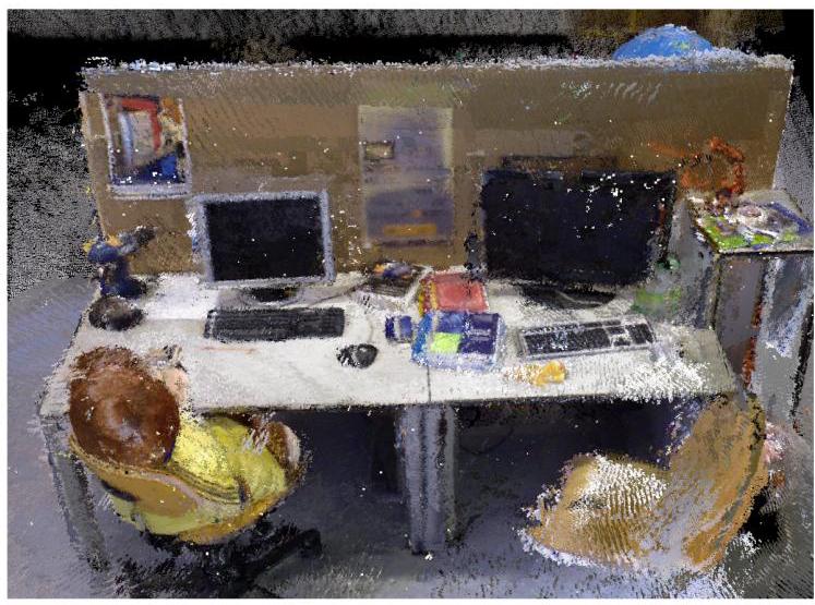
Fig. 5. UFOMap volumetric color mapping at $4\mathrm{mm}$ voxel size.

图5. 体素大小为 $4\mathrm{mm}$ 时的UFOMap(不明飞行物地图)体素彩色映射。

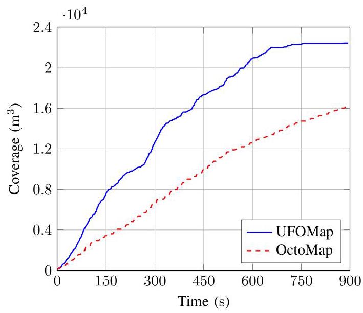
Fig. 6. Comparision of exploration progress between UFOMap and OctoMap in the power plant scenario.

图6. 发电厂场景中UFOMap(不明飞行物地图)和OctoMap(八叉地图)的探索进度比较。

The power plant scenario from the Gazebo model library ${}^3$ was used for the exploration test, seen in Fig. 1. $16\mathrm{cm}$ voxel size was used. As can be seen in Fig. 6, switching from OctoMap to UFOMap makes a significant difference to the exploration rate. UFOMap managed to finish the exploration after around $650\mathrm{s}$ , while OctoMap had completed $70\%$ of the exploration after $900\mathrm{s}$ , which was the maximum allowed time.

探索测试使用了Gazebo模型库(Gazebo model library)中的发电厂场景 ${}^3$，如图1所示。使用了 $16\mathrm{cm}$ 的体素大小。如图6所示，从八叉地图(OctoMap)切换到不明飞行物地图(UFOMap)对探索速率有显著影响。不明飞行物地图在大约 $650\mathrm{s}$ 后完成了探索，而八叉地图在 $900\mathrm{s}$(允许的最长时间)后仅完成了 $70\%$ 的探索。

We also investigated running the exploration without mu-texes, that is, allowing the mapping and the exploration sides simultaneous access to the map. Both OctoMap and UFOMap crashed. However, UFOMap did not crash when the indicator $i_a$ was used. As described in Section IV-B, this indicator turns off the automatic pruning, since nodes are not actually removed from the octree in this case.

我们还研究了在不使用互斥锁的情况下进行探索，即允许建图和探索端同时访问地图。八叉地图和不明飞行物地图都会崩溃。然而，当使用指标 $i_a$ 时，不明飞行物地图不会崩溃。如第四节B所述，该指标会关闭自动剪枝，因为在这种情况下节点实际上并未从八叉树中移除。

VII. CONCLUSION

七、结论

We present UFOMap, an open source framework for 3D mapping. UFOMap was built on OctoMap, which is one of the basic building blocks in a number of different robotics applications. Just like OctoMap, the underlying data structure is an octree. OctoMap only explicitly models occupied and free space, while UFOMap explicitly models occupied, free, and unknown space. This representation, together with the fact that every node in the octree stores indicators for what kind of space their children contains, results in a significant performance boost compared to OctoMap for use cases where unknown space is extensively used.

我们介绍了不明飞行物地图(UFOMap)，这是一个用于三维建图的开源框架。不明飞行物地图基于八叉地图(OctoMap)构建，八叉地图是许多不同机器人应用中的基本构建模块之一。与八叉地图一样，其底层数据结构是八叉树。八叉地图仅显式建模占用空间和空闲空间，而不明飞行物地图显式建模占用空间、空闲空间和未知空间。这种表示方式，再加上八叉树中的每个节点都存储了其孩子节点所包含空间类型的指标这一事实，使得在广泛使用未知空间的用例中，与八叉地图相比，性能有了显著提升。

Along with these improvements, we introduce new ways of integrating data into the octree. We show that this leads to significant reductions in the time to insert new measurement data, such as point clouds, into the map.

除了这些改进，我们还引入了将数据集成到八叉树中的新方法。我们表明，这显著减少了将新的测量数据(如点云)插入到地图中的时间。

The UFOMap mapping framework is freely available at https://github.com/danielduberg/UFOMap and can be easily integrated with robotics systems. It is written in $\mathrm{C}++$ and can be run as a standalone package or integrated into ROS [18].

不明飞行物地图建图框架可在https://github.com/danielduberg/UFOMap上免费获取，并且可以轻松集成到机器人系统中。它用 $\mathrm{C}++$ 编写，可以作为独立包运行，也可以集成到机器人操作系统(ROS)[18]中。

REFERENCES

参考文献

[1] I.-S. Kweon, M. Hebert, E. Krotkov, and T. Kanade, “Terrain mapping for a roving planetary explorer,” in IEEE International Conference on Robotics and Automation. IEEE, 1989, pp. 997-1002.

[1] I.-S. Kweon、M. Hebert、E. Krotkov和T. Kanade，“漫游行星探测器的地形测绘”，发表于电气与电子工程师协会国际机器人与自动化会议(IEEE International Conference on Robotics and Automation)，电气与电子工程师协会(IEEE)，1989年，第997 - 1002页。

[2] R. Triebel, P. Pfaff, and W. Burgard, “Multi-level surface maps for outdoor terrain mapping and loop closing,” in 2006 IEEE/RSJ international conference on intelligent robots and systems. IEEE, 2006, pp. 2276- 2282.

[2] R. Triebel、P. Pfaff和W. Burgard，“用于户外地形测绘和闭环检测的多级表面地图”，发表于2006年电气与电子工程师协会/日本机器人协会国际智能机器人与系统会议(2006 IEEE/RSJ international conference on intelligent robots and systems)，电气与电子工程师协会，2006年，第2276 - 2282页。

[3] D. Meagher, “Geometric modeling using octree encoding,” Computer graphics and image processing, vol. 19, no. 2, pp. 129-147, 1982.

[3] D. Meagher，“使用八叉树编码的几何建模”，《计算机图形学与图像处理》(Computer graphics and image processing)，第19卷，第2期，第129 - 147页，1982年。

[4] H. Oleynikova, A. Millane, Z. Taylor, E. Galceran, J. Nieto, and R. Siegwart, “Signed distance fields: A natural representation for both mapping and planning,” in RSS 2016 Workshop: Geometry and Beyond-Representations, Physics, and Scene Understanding for Robotics, 2016.

[4] H. Oleynikova、A. Millane、Z. Taylor、E. Galceran、J. Nieto和R. Siegwart，“有符号距离场:一种适用于建图和规划的自然表示方法”，发表于2016年机器人科学与系统研讨会(RSS 2016 Workshop: Geometry and Beyond - Representations, Physics, and Scene Understanding for Robotics)，2016年。

[5] A. Hornung, K. M. Wurm, M. Bennewitz, C. Stachniss, and W. Burgard, “OctoMap: An efficient probabilistic 3D mapping framework based on octrees,” Autonomous Robots, vol. 34, no. 3, pp. 189-206, 2013.

[5] A. Hornung、K. M. Wurm、M. Bennewitz、C. Stachniss和W. Burgard，“八叉地图:一种基于八叉树的高效概率三维建图框架”，《自主机器人》(Autonomous Robots)，第34卷，第3期，第189 - 206页，2013年。

[6] A. Bircher, M. Kamel, K. Alexis, H. Oleynikova, and R. Siegwart, “Receding horizon “next-best-view” planner for $3\mathrm{d}$ exploration,” in Robotics and Automation (ICRA), 2016 IEEE International Conference on. IEEE, 2016, pp. 1462-1468.

[6] A. Bircher、M. Kamel、K. Alexis、H. Oleynikova和R. Siegwart，“用于 $3\mathrm{d}$ 探索的滚动时域‘下一最佳视角’规划器”，发表于2016年电气与电子工程师协会国际机器人与自动化会议(Robotics and Automation (ICRA), 2016 IEEE International Conference on)，电气与电子工程师协会，2016年，第1462 - 1468页。

[7] M. Selin, M. Tiger, D. Duberg, F. Heintz, and P. Jensfelt, “Efficient Autonomous Exploration Planning of Large-Scale 3-D Environments,” IEEE Robotics and Automation Letters, vol. 4, no. 2, pp. 1699-1706, 2019.

[7] M. Selin、M. Tiger、D. Duberg、F. Heintz和P. Jensfelt，“大规模三维环境的高效自主探索规划”，《电气与电子工程师协会机器人与自动化快报》(IEEE Robotics and Automation Letters)，第4卷，第2期，第1699 - 1706页，2019年。

[8] F. S. Barbosa, D. Duberg, P. Jensfelt, and J. Tumova, “Guiding Autonomous Exploration With Signal Temporal Logic,” IEEE Robotics and Automation Letters, vol. 4, no. 4, pp. 3332-3339, 2019.

[8] F. S. Barbosa、D. Duberg、P. Jensfelt和J. Tumova，“用信号时序逻辑引导自主探索”，《电气与电子工程师协会机器人与自动化快报》，第4卷，第4期，第3332 - 3339页，2019年。

[9] L. M. Schmid, M. Pantic, R. Khanna, L. Ott, R. Siegwart, and J. Nieto, “An Efficient Sampling-based Method for Online Informative Path Planning in Unknown Environments,” IEEE Robotics and Automation Letters, 2020.

[9] L. M. 施密德(L. M. Schmid)、M. 潘蒂奇(M. Pantic)、R. 坎纳(R. Khanna)、L. 奥特(L. Ott)、R. 西格沃特(R. Siegwart)和 J. 涅托(J. Nieto)，《未知环境中基于在线信息路径规划的高效采样方法》，《IEEE 机器人与自动化快报》，2020 年。

[10] M. Pivtoraiko, D. Mellinger, and V. Kumar, “Incremental micro-UAV motion replanning for exploring unknown environments,” in 2013 IEEE International Conference on Robotics and Automation, 2013, pp. 2452- 2458.

[10] M. 皮夫托拉伊科(M. Pivtoraiko)、D. 梅林杰(D. Mellinger)和 V. 库马尔(V. Kumar)，《用于探索未知环境的微型无人机增量式运动重规划》，收录于 2013 年 IEEE 国际机器人与自动化会议论文集，2013 年，第 2452 - 2458 页。

[11] J. Chen, T. Liu, and S. Shen, “Online generation of collision-free trajectories for quadrotor flight in unknown cluttered environments,” in 2016 IEEE International Conference on Robotics and Automation (ICRA), 2016, pp. 1476-1483.

[11] J. 陈(J. Chen)、T. 刘(T. Liu)和 S. 沈(S. Shen)，《未知杂乱环境中四旋翼飞行器无碰撞轨迹的在线生成》，收录于 2016 年 IEEE 国际机器人与自动化会议(ICRA)论文集，2016 年，第 1476 - 1483 页。

[12] Y. Roth-Tabak and R. Jain, “Building an environment model using depth information,” Computer, vol. 22, no. 6, pp. 85-90, 1989.

[12] Y. 罗斯 - 塔巴克(Y. Roth - Tabak)和 R. 贾因(R. Jain)，《利用深度信息构建环境模型》，《计算机》，第 22 卷，第 6 期，第 85 - 90 页，1989 年。

[13] M. Nießner, M. Zollhöfer, S. Izadi, and M. Stamminger, “Real-time 3D reconstruction at scale using voxel hashing,” ACM Transactions on Graphics (ToG), vol. 32, no. 6, p. 169, 2013.

[13] M. 尼斯纳(M. Nießner)、M. 佐尔霍费尔(M. Zollhöfer)、S. 伊扎迪(S. Izadi)和 M. 施塔明格(M. Stamminger)，《使用体素哈希进行大规模实时 3D 重建》，《ACM 图形学汇刊》(ToG)，第 32 卷，第 6 期，第 169 页，2013 年。

[14] H. Oleynikova, Z. Taylor, M. Fehr, R. Siegwart, and J. Nieto, “Voxblox: Incremental $3\mathrm{d}$ euclidean signed distance fields for on-board mav planning,” in 2017 leee/rsj International Conference on Intelligent Robots and Systems (iros), 2017, pp. 1366-1373.

[14] H. 奥列尼科娃(H. Oleynikova)、Z. 泰勒(Z. Taylor)、M. 费尔(M. Fehr)、R. 西格沃特(R. Siegwart)和 J. 涅托(J. Nieto)，《Voxblox:用于机载无人机规划的增量式 $3\mathrm{d}$ 欧几里得有符号距离场》，收录于 2017 年 IEEE/RSJ 国际智能机器人与系统会议(IROS)论文集，2017 年，第 1366 - 1373 页。

[15] G. M. Morton, “A computer oriented geodetic data base and a new technique in file sequencing,” 1966.

[15] G. M. 莫顿(G. M. Morton)，《面向计算机的大地测量数据库及文件排序新技术》，1966 年。

[16] L. Stocco and G. Schrack, “Integer dilation and contraction for quadtrees and octrees,” in IEEE Pacific Rim Conference on Communications, Computers, and Signal Processing. Proceedings, 1995, pp. 426-428.

[16] L. 斯托科(L. Stocco)和 G. 施拉克(G. Schrack)，《四叉树和八叉树的整数膨胀与收缩》，收录于 IEEE 环太平洋通信、计算机与信号处理会议论文集，1995 年，第 426 - 428 页。

[17] J. Amanatides, A. Woo, and others, “A fast voxel traversal algorithm for ray tracing,” in Eurographics, vol. 87, no. 3, 1987, pp. 3-10.

[17] J. 阿玛纳蒂德斯(J. Amanatides)、A. 吴(A. Woo)等人，《用于光线追踪的快速体素遍历算法》，收录于《欧洲图形学》，第 87 卷，第 3 期，1987 年，第 3 - 10 页。

[18] M. Quigley, K. Conley, B. Gerkey, J. Faust, T. Foote, J. Leibs, R. Wheeler, and A. Y. Ng, “{ROS}: an open-source Robot Operating System,” in ICRA workshop on open source software, vol. 3, no. 3.2. Kobe, Japan, 2009, p. 5.

[18] M. 奎格利(M. Quigley)、K. 康利(K. Conley)、B. 杰基(B. Gerkey)、J. 福斯特(J. Faust)、T. 富特(T. Foote)、J. 莱布斯(J. Leibs)、R. 惠勒(R. Wheeler)和 A. Y. 吴(A. Y. Ng)，《ROS:开源机器人操作系统》，收录于 ICRA 开源软件研讨会论文集，第 3 卷，第 3.2 期。日本神户，2009 年，第 5 页。

[19] C. Connolly, “The determination of next best views,” in Robotics and automation. Proceedings. 1985 IEEE international conference on, vol. 2. IEEE, 1985, pp. 432-435.

[19] C. 康诺利(C. Connolly)，《确定下一个最佳视角》，收录于《机器人与自动化会议论文集》。1985 年 IEEE 国际会议，第 2 卷。IEEE，1985 年，第 432 - 435 页。

[20] J. Sturm, N. Engelhard, F. Endres, W. Burgard, and D. Cremers, “A benchmark for the evaluation of RGB-D SLAM systems,” in 2012 IEEE/RSJ Ineternational Conference on Intelligent Robots and Systems, 2012, pp. 573-580.

[20] J. 施图尔姆(J. Sturm)、N. 恩格尔哈德(N. Engelhard)、F. 恩德斯(F. Endres)、W. 布尔加德(W. Burgard)和 D. 克雷默斯(D. Cremers)，《RGB - D 同步定位与地图构建(SLAM)系统评估基准》，收录于 2012 年 IEEE/RSJ 国际智能机器人与系统会议论文集，2012 年，第 573 - 580 页。

---

${}^3$ https://bitbucket.org/osrf/gazebo_models/src

${}^3$ https://bitbucket.org/osrf/gazebo_models/src

---