Ensemble methods --Bagging meta-estimator

集成学习介绍
通过使用对多个基学习器的整合来达到超过每个学习器的预测和稳定性。
主要分为两种思想：
averaging methods：个体学习器之间存在强依赖关系、必须串行生成，可以减小方差；例如Boosting
boosting methods：个体学习器之间不存在强依赖关系，可同时生成并行化方法；例如Bagging, RandomForest

1.Bagging meta-estimator
集成算法中，bagging通过对基于原始训练集的随机样本的黑盒学习器的结果进行整合，组成最后的预测结果。这些方法通过使用在构建过程中的随机化来减少基学习器的方差，然后通过投票或平均做出最后的预测。bagging不用必须适配每一个学习器，它提供了减少过拟合的方法，比较复杂模型，相反boosting比较适合简单模型。
在sklearn中，bagging通过统一的BaggingClassifier (回归用 BaggingRegressor)，采用用户自定义的一些参数来产生随机输入集。特别是max_samples和max_features来控制样本的大小（一个控制样本的数量，一个控制特征的数量），另外bootstrap和bootstrap_features分别控制样本和特征是不是有放回地采样。根据bagging的原理每次采样都是随机地，因此可能会有一些样本没有被用来训练，这一部分样本就可以被用来计算范化误差，通过设置 oob_score=True。

参数：
———-
base_estimator : object or None, optional (default=None)
The base estimator to fit on random subsets of the dataset.
If None, then the base estimator is a decision tree.
要拟合随机数据集的基学习器，如果是NONE,就是决策树

n_estimators : int, optional (default=10)
    The number of base estimators in the ensemble.
    基学习器的数量

max_samples : int or float, optional (default=1.0)
    The number of samples to draw from X to train each base estimator.
    要训练每个学习器的样本个数
        - If int, then draw `max_samples` samples.
        - If float, then draw `max_samples * X.shape[0]` samples.

max_features : int or float, optional (default=1.0)
    要训练每个学习器的特征个数
    The number of features to draw from X to train each base estimator.
        - If int, then draw `max_features` features.
        - If float, then draw `max_features * X.shape[1]` features.

bootstrap : boolean, optional (default=True)
    样本是否有放回抽取
    Whether samples are drawn with replacement.

bootstrap_features : boolean, optional (default=False)
    Whether features are drawn with replacement.
    特征是否有放回抽取

oob_score : bool
    Whether to use out-of-bag samples to estimate
    the generalization error.
    是否使用“包外”样本计算范化误差

warm_start : bool, optional (default=False)
    When set to True, reuse the solution of the previous call to fit
    and add more estimators to the ensemble, otherwise, just fit
    a whole new ensemble.
    当设置成True时，将重复使用当前的学习器，增加更多的学习器到集成中，否则仅仅拟合一整个新的学习器

    .. versionadded:: 0.17
       *warm_start* constructor parameter.

n_jobs : int, optional (default=1)
    The number of jobs to run in parallel for both `fit` and `predict`.
    并行的线程数，默认为1；如果设置成-1，就是核数
    If -1, then the number of jobs is set to the number of cores.

random_state : int, RandomState instance or None, optional (default=None)
    If int, random_state is the seed used by the random number generator;
    If RandomState instance, random_state is the random number generator;
    If None, the random number generator is the RandomState instance used
    by `np.random`.
    随机种子，默认为None,即np.random。

verbose : int, optional (default=0)
    Controls the verbosity of the building process.
    ？？？
属性
----------
base_estimator_ : list of estimators
    The base estimator from which the ensemble is grown.
    要集成的基学习器

estimators_ : list of estimators
    被拟合的学习器
    The collection of fitted base estimators.

estimators_samples_ : list of arrays
    The subset of drawn samples (i.e., the in-bag samples) for each base
    estimator.
    每个基学习器的样本集合

estimators_features_ : list of arrays
    The subset of drawn features for each base estimator.
    每个基学习器的特征集合

classes_ : array of shape = [n_classes]
    The classes labels.
    所有类的标签

n_classes_ : int or list
    The number of classes.
    所有类的数目
oob_score_ : float
    Score of the training dataset obtained using an out-of-bag estimate.
    使用包外估计得到的训练集的得分
oob_decision_function_ : array of shape = [n_samples, n_classes]
    Decision function computed with out-of-bag estimate on the training
    set. If n_estimators is small it might be possible that a data point
    was never left out during the bootstrap. In this case,
    `oob_decision_function_` might contain NaN.
    训练集上使用包外估计的计算函数；如果学习器数比较少，可能样本点不会被剩下，这
时“oob_decision_function_”就被设置成NaN。

方法：
decision_function(X) Average of the decision functions of the base classifiers.
fit(X, y[, sample_weight]) Build a Bagging ensemble of estimators from the training set (X, y).
get_params([deep]) Get parameters for this estimator.
predict(X) Predict class for X.
predict_log_proba(X) Predict class log-probabilities for X.
predict_proba(X) Predict class probabilities for X.
score(X, y[, sample_weight]) Returns the mean accuracy on the given test data and labels.
set_params(**params) Set the parameters of this estimator.

decision_function(X)[source]
基分类器的决定函数的平均值
Average of the decision functions of the base classifiers.
参数:
X : {array-like, sparse matrix} of shape = [n_samples, n_features]
The training input samples. Sparse matrices are accepted only if they are supported by the base estimator.
X:输入训练样本，shape=[n_samples, n_features]，为矩阵或稀疏矩阵；当为稀疏矩阵的时候只有被基学习器接受才可以。
返回值:
score : array, shape = [n_samples, k]
一个shape = [n_samples, k]的得分矩阵
The decision function of the input samples. The columns correspond to the classes in sorted order, as they appear in the attribute classes_. Regression and binary classification are special cases with k == 1, otherwise k==n_classes.
输入样本的决定函数。列是按它们出现的属性类中排序后的类。回归和二分类被指定k==1,其它k==n_classes

fit(X, y, sample_weight=None)[source]
Build a Bagging ensemble of estimators from the training
fit函数用来建立一个基于训练集的bagging集成学习器
set (X, y).
参数:
X：一个shape = [n_samples, n_features]的输入训练集矩阵
y:shape = [n_samples]的一个回归中真实值的标签矩阵
sample_weight : shape = [n_samples]的权重矩阵，或者为None.如果是None,样本将会取相等权重。注意这仅仅是当基学习器支持样本权重的情况下。
返回值:
self : object
Returns self.

get_params(deep=True)[source]
得到这个学习器的参数
Parameters:
deep: boolean, optional :
如果是True，则返回这个学习器的参数和子对象的参数
返回值: 参数名以及参数值
params : mapping of string to any
Parameter names mapped to their values.

predict(X)[source]
X的预测类
输入样本的预测类将按照被预测平均值最高的类被预测。如果基学习器没有执行predict_proba方法，它将会采用投票的方法。
参数:
X : {array-like, sparse matrix} of shape = [n_samples, n_features]
Returns:
y : array of shape = [n_samples] 被预测的类

predict_log_proba(X)[source]
X被预测类的log-p值；在集成中基学习器的被预测类的p值得log（对数）值
参数:
X : {array-like, sparse matrix} of shape = [n_samples, n_features]
Returns:
p : array of shape = [n_samples, n_classes]
The class log-probabilities of the input samples. The order of the classes corresponds to that in the attribute classes_.
p:shape = [n_samples, n_classes]的一个矩阵。相应的类与属性中classes_的顺序相对应。

predict_proba(X)[source]
Predict class probabilities for X.
The predicted class probabilities of an input sample is computed as the mean predicted class probabilities of the base estimators in the ensemble. If base estimators do not implement a predict_proba method, then it resorts to voting and the predicted class probabilities of a an input sample represents the proportion of estimators predicting each class.
X的预测类的p值
输入样本的预测类将按照被预测平均值最高的类被预测。如果基学习器没有执行predict_proba方法，它将会采用投票的方法，对于每一个输入样本的预测类的可能性p表示预测为每一类的学习器的比例。
Parameters:
X : {array-like, sparse matrix} of shape = [n_samples, n_features]
返回值:
p : array of shape = [n_samples, n_classes]
The class probabilities of the input samples. The order of the classes corresponds to that in the attribute classes_.
X被预测类的p值；在集成中基学习器的被预测类的p值。

score(X, y, sample_weight=None)[source]
Returns the mean accuracy on the given test data and labels.
In multi-label classification, this is the subset accuracy which is a harsh metric since you require for each sample that each label set be correctly predicted.
返回给定测试集和标签的准确度。在多标签分类中，这个子集被严格度量，因为我们要求每个样本预测结果必须与标签完全相同
参数:
X : array-like, shape = (n_samples, n_features)
测试样本X
y : array-like, shape = (n_samples) or (n_samples, n_outputs)
X的真实标签
sample_weight : array-like, shape = [n_samples], optional
Sample weights.
返回值:
score : float
Mean accuracy of self.predict(X) wrt. y.

set_params(**params)[source]
设置学习器的参数.
该方法作用于学习器和嵌套对象。前者有__形式的参数，因此可以更新每一个嵌套对象
The method works on simple estimators as well as on nested objects (such as pipelines). The former have parameters of the form __ so that it’s possible to update each component of a nested object.
Returns: self :

2.案例说明–Single estimator versus bagging: bias-variance decomposition
2.1 结果说明
这个例子阐述比较了单个学习器与bagging的期望均方差的偏差-方差分解。在回归中，一个学习器的期望均方差可以分解成偏差$bias$，方差$vars$和误差$error$。偏差表示的是学习器的预测值与最优预测值之间的差；方差表示的是学习器拟合一个问题的不同实例预测结果的可变性，而误差是数据内部不可消除的因素。

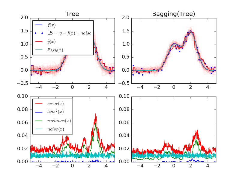
左上方的图描述了一个对于随机数据集的单个决策树的预测的一维回归问题（深红色点），也描述了其它单个决策树对于随机实例的预测（浅红色点）。直观上来看，方差对应学习器的波动的宽度，方差越大，则学习器对训练集X很小的变动越是敏感；偏差项是指学习器的平均预测值（浅蓝）与模型最优概率（深蓝）之间的不同，对应的是浅蓝色和深蓝色线之间的不同，对于这个问题我没看到两者靠得很近，说明偏差非常低，方差比较大。
左下方的图画出了一个决策树期望均方差的分解图，这幅图表明偏差项（蓝）低，方差项（绿）高，也表明误差项似乎是一个约0.01的常数。
右面两个图是决策树bagging集成的图。这两幅图中看以看出偏差项比当前值要大，右上图中平均预测值与最优模型之间的差比较大（例如x=2时）。在右下图中，偏差曲线比左下图高一点。方差项，右图明显变窄，说明方差更低，右下图证明了这一点。总之，偏差-方差分解不再相同，权衡一下认为bagging比较好：平均化拟合决策树虽然略增加了偏差，但是大大减少了方差，这将导致更低的均方差（比较下面两个图的红线）。脚本输出也证明了这一点。bagging集成的总误差比单个决策树的总误差要低，这主要就是因为减少了方差。
2.2 放“马”出来

print(__doc__)

# Author: Gilles Louppe <g.louppe@gmail.com>
# License: BSD 3 clause

import numpy as np
import matplotlib.pyplot as plt

from sklearn.ensemble import BaggingRegressor
from sklearn.tree import DecisionTreeRegressor

# Settings
n_repeat = 50       # Number of iterations for computing expectations
n_train = 50        # Size of the training set
n_test = 1000       # Size of the test set
noise = 0.1         # Standard deviation of the noise
np.random.seed(0)

# Change this for exploring the bias-variance decomposition of other
# estimators. This should work well for estimators with high variance (e.g.,
# decision trees or KNN), but poorly for estimators with low variance (e.g.,
# linear models).
estimators = [("Tree", DecisionTreeRegressor()),
              ("Bagging(Tree)", BaggingRegressor(DecisionTreeRegressor()))]

n_estimators = len(estimators)

# Generate data
def f(x):
    x = x.ravel()

    return np.exp(-x ** 2) + 1.5 * np.exp(-(x - 2) ** 2)

def generate(n_samples, noise, n_repeat=1):
    X = np.random.rand(n_samples) * 10 - 5
    X = np.sort(X)

    if n_repeat == 1:
        y = f(X) + np.random.normal(0.0, noise, n_samples)
    else:
        y = np.zeros((n_samples, n_repeat))

        for i in range(n_repeat):
            y[:, i] = f(X) + np.random.normal(0.0, noise, n_samples)

    X = X.reshape((n_samples, 1))

    return X, y

X_train = []
y_train = []

for i in range(n_repeat):
    X, y = generate(n_samples=n_train, noise=noise)
    X_train.append(X)
    y_train.append(y)

X_test, y_test = generate(n_samples=n_test, noise=noise, n_repeat=n_repeat)

# Loop over estimators to compare
for n, (name, estimator) in enumerate(estimators):
    # Compute predictions
    y_predict = np.zeros((n_test, n_repeat))

    for i in range(n_repeat):
        estimator.fit(X_train[i], y_train[i])
        y_predict[:, i] = estimator.predict(X_test)

    # Bias^2 + Variance + Noise decomposition of the mean squared error
    y_error = np.zeros(n_test)

    for i in range(n_repeat):
        for j in range(n_repeat):
            y_error += (y_test[:, j] - y_predict[:, i]) ** 2

    y_error /= (n_repeat * n_repeat)

    y_noise = np.var(y_test, axis=1)
    y_bias = (f(X_test) - np.mean(y_predict, axis=1)) ** 2
    y_var = np.var(y_predict, axis=1)

    print("{0}: {1:.4f} (error) = {2:.4f} (bias^2) "
          " + {3:.4f} (var) + {4:.4f} (noise)".format(name,
                                                      np.mean(y_error),
                                                      np.mean(y_bias),
                                                      np.mean(y_var),
                                                      np.mean(y_noise)))

    # Plot figures
    plt.subplot(2, n_estimators, n + 1)
    plt.plot(X_test, f(X_test), "b", label="$f(x)$")
    plt.plot(X_train[0], y_train[0], ".b", label="LS ~ $y = f(x)+noise$")

    for i in range(n_repeat):
        if i == 0:
            plt.plot(X_test, y_predict[:, i], "r", label="$\^y(x)$")
        else:
            plt.plot(X_test, y_predict[:, i], "r", alpha=0.05)

    plt.plot(X_test, np.mean(y_predict, axis=1), "c",
             label="$\mathbb{E}_{LS} \^y(x)$")

    plt.xlim([-5, 5])
    plt.title(name)

    if n == 0:
        plt.legend(loc="upper left", prop={"size": 11})

    plt.subplot(2, n_estimators, n_estimators + n + 1)
    plt.plot(X_test, y_error, "r", label="$error(x)$")
    plt.plot(X_test, y_bias, "b", label="$bias^2(x)$"),
    plt.plot(X_test, y_var, "g", label="$variance(x)$"),
    plt.plot(X_test, y_noise, "c", label="$noise(x)$")

    plt.xlim([-5, 5])
    plt.ylim([0, 0.1])

    if n == 0:
        plt.legend(loc="upper left", prop={"size": 11})

plt.show()

参考文献：

[1] T. Hastie, R. Tibshirani and J. Friedman, “Elements of Statistical Learning”, Springer, 2009.