


简介
score matching算法是一种求解概率密度函数的参数的算法。
在很多情况下,概率密度函数可以表示为:
p
(
ξ
;
θ
)
=
1
Z
(
θ
)
q
(
ξ
;
θ
)
p(\xi;\theta)=\frac{1}{Z(\theta)}q(\xi;\theta)
p(ξ;θ)=Z(θ)1q(ξ;θ)
假设我们知道
q
q
q的解析表达式,但是因为
Z
Z
Z的计算需要积分计算,并不能简单地计算
Z
Z
Z。
score matching算法通过绕开归一化常数
Z
Z
Z,求解概率密度函数的参数
θ
\theta
θ。
Score Function
为了去掉
Z
Z
Z,我们定义分数函数score function
ψ
(
ξ
;
θ
)
\psi(\xi;\theta)
ψ(ξ;θ):
ψ
(
ξ
;
θ
)
=
(
∂
log
p
(
ξ
;
θ
)
∂
ξ
1
⋮
∂
log
p
(
ξ
;
θ
)
∂
ξ
n
)
=
(
ψ
1
(
ξ
;
θ
)
⋮
ψ
n
(
ξ
;
θ
)
)
=
∇
ξ
log
p
(
ξ
;
θ
)
\psi(\xi;\theta)=\left (\begin{array}{c} \frac{\partial\log p(\xi;\theta)}{\partial \xi_1} \\ \vdots \\ \frac{\partial\log p(\xi;\theta)}{\partial \xi_n} \\ \end{array}\right)=\left (\begin{array}{c} \psi_1(\xi;\theta) \\ \vdots \\ \psi_n(\xi;\theta) \\ \end{array}\right)=\nabla_\xi \log p(\xi;\theta)
ψ(ξ;θ)=
∂ξ1∂logp(ξ;θ)⋮∂ξn∂logp(ξ;θ)
=
ψ1(ξ;θ)⋮ψn(ξ;θ)
=∇ξlogp(ξ;θ)
因为
Z
(
θ
)
Z(\theta)
Z(θ)和
ξ
\xi
ξ无关,通过score function可以去掉
Z
(
θ
)
Z(\theta)
Z(θ),即score function只依赖
q
q
q
ψ
(
ξ
;
θ
)
=
∇
ξ
log
q
(
ξ
;
θ
)
\psi(\xi;\theta)=\nabla_\xi\log q(\xi;\theta)
ψ(ξ;θ)=∇ξlogq(ξ;θ)
另外,用 ψ x ( ⋅ ) = ∇ ξ log p x ( ⋅ ) \psi_x(\cdot)=\nabla_\xi \log p_x(\cdot) ψx(⋅)=∇ξlogpx(⋅)表示观测数据的score function。
求解方法
score matching算法通过最小化模型分数函数
ψ
(
ξ
;
θ
)
\psi(\xi;\theta)
ψ(ξ;θ)和数据分数函数
ψ
x
(
ξ
;
θ
)
\psi_x(\xi;\theta)
ψx(ξ;θ)的平方差的期望来得到参数
θ
\theta
θ。该期望的定义如下:
J
(
θ
)
=
1
2
∫
ξ
∈
R
n
p
x
(
ξ
)
∥
ψ
(
ξ
;
θ
)
−
ψ
x
(
ξ
;
θ
)
∥
2
d
ξ
J(\theta)=\frac{1}{2}\int_{\xi\in \mathbb{R}^n}p_x(\xi)\|\psi(\xi;\theta)-\psi_x(\xi;\theta)\|^2d\xi
J(θ)=21∫ξ∈Rnpx(ξ)∥ψ(ξ;θ)−ψx(ξ;θ)∥2dξ
最小化上面的期望将得到
θ
\theta
θ的score matching估计量(estimator):
θ
^
=
argmin
J
(
θ
)
\hat{\theta}=\text{argmin}J(\theta)
θ^=argminJ(θ)
因为score function不含有
Z
Z
Z,优化
J
(
θ
)
J(\theta)
J(θ)可以去掉对
Z
Z
Z的计算。但值得注意的是,直接优化
J
(
θ
)
J(\theta)
J(θ)依然很难,因为数据分数函数
ψ
x
(
ξ
;
θ
)
\psi_x(\xi;\theta)
ψx(ξ;θ)的计算是一个非参数估计问题(non-parametric estimation problem)。
但是可以证明
J
(
θ
)
J(\theta)
J(θ)可以重写成没有数据分数函数的形式:
J
(
θ
)
=
∫
ξ
∈
R
n
p
x
(
ξ
)
∑
i
=
1
n
[
∂
i
ψ
i
(
ξ
;
θ
)
+
1
2
ψ
i
(
ξ
;
θ
)
2
]
d
ξ
+
c
o
n
s
t
J(\theta)=\int_{\xi\in \mathbb{R}^n}p_x(\xi)\sum_{i=1}^n[\partial_i\psi_i(\xi;\theta)+\frac{1}{2}\psi_i(\xi;\theta)^2]d\xi+const
J(θ)=∫ξ∈Rnpx(ξ)i=1∑n[∂iψi(ξ;θ)+21ψi(ξ;θ)2]dξ+const
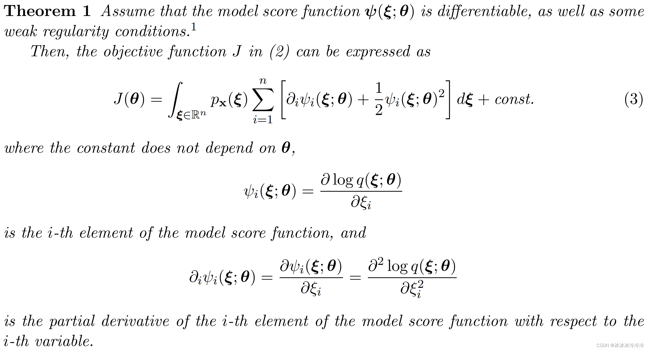
下面是论文中给出的完整定理。
现实中,假设我们有
T
T
T个观测值
x
(
1
)
,
…
,
x
(
T
)
x(1),\ldots,x(T)
x(1),…,x(T)。根据大数定理,期望可以用平均数表示,
J
J
J则表示成
J
~
(
θ
)
=
1
T
∑
t
=
1
T
∑
i
=
1
n
[
∂
i
ψ
i
(
x
(
t
)
;
θ
)
+
1
2
ψ
i
(
x
(
t
)
;
θ
)
2
]
d
ξ
+
c
o
n
s
t
\tilde{J}(\theta)=\frac{1}{T}\sum_{t=1}^T\sum_{i=1}^n[\partial_i\psi_i(x(t);\theta)+\frac{1}{2}\psi_i(x(t);\theta)^2]d\xi+const
J~(θ)=T1t=1∑Ti=1∑n[∂iψi(x(t);θ)+21ψi(x(t);θ)2]dξ+const
可以证明,如果
θ
^
\hat{\theta}
θ^是
J
~
\tilde{J}
J~的全局最优解,那么估计量
θ
^
\hat{\theta}
θ^将具有一致性(consistent)。
具有一致性的估计量是渐进无偏(asymptotic unbiasedness)的。
emm
从统计学的角度理解score matching。score matching就是要从观测数据估计出总体的未知参数。 θ ^ \hat{\theta} θ^是估计量, θ \theta θ是被估计量。估计量需要具有一些性质才是好的估计量。这里 θ ^ \hat{\theta} θ^在一定条件下具有一致性(consistent)。
参考
[1]: Estimation of Non-Normalized Statistical Models by Score Matching


 1676
1676

 被折叠的 条评论
为什么被折叠?
被折叠的 条评论
为什么被折叠?
 到【灌水乐园】发言


