Image Sampling and Nyquist Theorem (summary)

This article is the summary of 1D, 2D sampling, convolution and Nyquist Theorem from the textbook Digital Image Processing Third Edition by Refael C. Gonzalez, Richard E. Woods., and the course of “Fundamentals of DigitalImage and Video Processing” by AT&T Professor Aggelos K. Katasaggelos, Departmentof Electrical Engineering and Computer Science, Northwestern University.

1.Overview

(1) Sampling

Sampling is the operation of turning a continuous signal into a discrete one.

Sampling is needed in being able to bring a continuous signal into the discrete world, so that it can be processed by a computer. In most cases they're also interested in bringing the discrete signal back to the continuous world. So that we can see it (for example, an image inspatial domain), or so that we're able to hear it (for examplem, a voice signal).

(2) The fundamental question

The fundamental question, therefore, when samplingis performed, is under what conditions can we move back and forth between the continuous and discrete worlds,without loss of information. Or,under what conditions we can reconstruct the continuous signal from its samples.

(3) Nyquist Theorem

The Nyquist Theorem: a continuous signal can be reconstructed from its samplesif it is sampled with frequency at least twice as large as the highest frequencyof the signal in each dimension.

We derive the theorem in 2D. However, it'sstraightforward extension of the 1D subject theorem. And it can also beextended in similar way to dimensions higher than two. Actually, in two andhigher dimensions, there is more freedom in preforming periodic sampling.

We'll only cover here rectangular periodic sampling, but one could use, for example, hexagonal periodic sampling in 2D. Sampling provides the intuition in understanding what happens when we sample now the continuous Fourier domain. It leads to the definition of the discrete Fourier series. And also the definition of the discrete Fourier transform.

2. 1D sampling

(1) Unit impulse

A unit impulse of a continuous variable t located at t=0, denoted δ(t)

And is constrained also to satisfy the identity

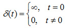
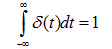
Physically, if we interpret t as time, an impulse may be viewed as a spike of infinity amplitude and zero duration, having unit area. An impulse has the so-called sifting property with respect to integration

(2) Unit discrete impulse

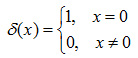
Let x representa discrete variable. The  unit discrete impulse,  δ(x), is defined as

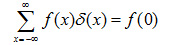
The sifting property for discrete variables has the form

Or more generally using a discrete impulse located at x=x₀,

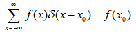
The sifting property simply yields the value of the function at the location of the impulse. The figure below shows the discrete impulse diagram matically. Unlike its continuous counter part, the discrete impulse is an ordinary function.

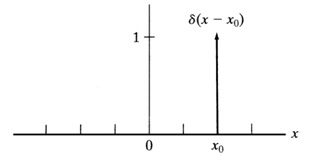
Fig.1 A unit discrete impulse located at x=x₀

(3) Impulse train

The impulse train defined as the sum of infinitely many periodic impulse △T units apart:

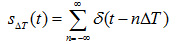
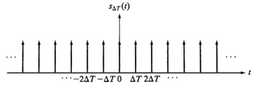
Fig.2 Impulse train

The Fourier transform of the impulse train is

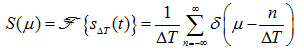
This fundamental result tells us that the Fourier transform of an impulse train with period △T is also an impulse train, whose period is 1/△T.

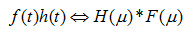
(4) Convolution Theorem

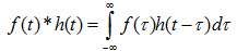
In this discussion, we are interested in theconvolution of two continuous function, f(t) and  h(t), of one continuous variable, t,so we have to use integration instead of a summation. The convolution of these two functions, denoted as before by the *, is defined as

The Fourier transform of the convolution above is 

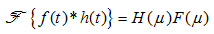
In other words, f(t) * h(t) and H(μ)F(μ) are a Fourier transform pair. This result is one-half of the convolution theorem and is written as

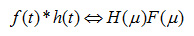
Following a similar development would result in the other half of the convolution theorem:

Which states that convolution in the frequency domain is an alogous to multiplication in the spatial domain, the two being related by the forward and inverse Fourier transforms, respectively. The convolution theorem is the foundation of the filtering in the frequency domain.

(5) Sampling and the Fourier Transform of Sampled Functions

Continuous functions have to be convertedinto a sequence of discrete values before they can be processed in a computer. This is accomplished by using sampling and quantization.

Consider a continuous function f(t), that we wish to sample at uniform intervals ( △T) of the independent variable  t. we assume that the function extends from –∞ to  +∞ with respect to  t. One way to model sampling is to multiply  f(t) by a sampling function equal to atrain of impulse △T units apart. The sampled function can be written as:

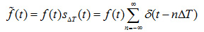
Each component of this summation is animpulse weighted by the value of f(t) at the location of the impulse, as Fig.3(c) shows below. And an arbitrary sample in the sequence is given by 

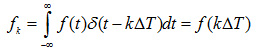
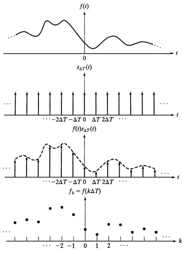
Fig.3 1D sampling of a continuous function

The Fourier Transform of Sampled Functions

Let F(μ) denoted the Fourier transform of a continuous function  f(t).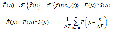

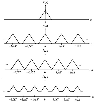
The summation in the equation shows that the Fourier transform of the sampled funciton is a infinite, periodic sequence of copies of  F ( μ ).

Fig.4(a) Fourier transform of a band-limited function (Fourier transform of theoriginal signal). (b)-(d) Transforms of the corresponding sampledfunction under the conditions of over-sampling, critically-sampling, andunder-sampling, respectively.

3. Sampling theorem

(1) Critically-sampling

A function whose Fourier transform is zerofor values of frequencies outside a finite interval (band) [-μ_max, μ_max] about the origin is called a band-limited function. Fig.5 is a more detailed view of the transformof a critically-sampled function shown in Fig.4(c). A lower value of 1/△T would cause the periods in F~(μ) to merge; a higher value would provide a clean separation between the periods. So the sampling at the rate of 1/△T is called critically-sampling.

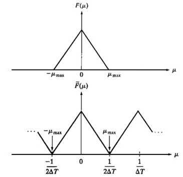
Fig.5 Transform resulting from critically sampling the same function

(2) Nyquist rate

We can recover f(t) from its sampled version if we can isolate a copy of F(μ) from the periodic sequence of copies of this function contained in F~(μ), the transform of the sampled function F~(t).

Therefore, all we need is one complete period to characterize the entire transform. This implies that we can recover f(t) from that signal period by using the inverse Fourier transform.

Extracting from F~(μ) a single period that is equal to F(μ) is possible if the separation between copies is sufficient. In terms of Fig.5(b), sufficient separation is guaranteed if 1/2△T>μ_max or 

4. 2D sampling

(1) The original image in the spatial domain and spectrum domain

So assume that we have an analog image like the one shown here, such an image can appear for example on a positive photographic field.

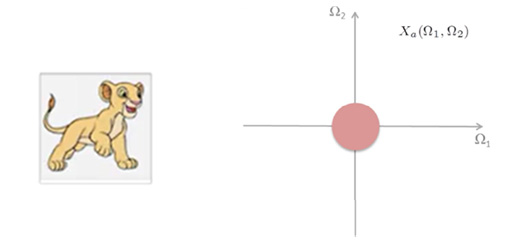
Fig.6 The original image in spatial domain and frequency domain 

Again I present the signal in the frequency domain, and here is the spectrum of the analog signal X_a(Ω₁,Ω₂). What we show here is really the region of support of this spectrum and not that shape of this spectrum itself, but it's not relevant the shape forthe discussion that follows.

(2) 2D sampled image and its frequency spectrum

I want now to represent this image by discrete sample. So, I super-impose a grid that's shown here, and only keep the values of the image at the grid points. So the digital image would end up with is the one shown here. And there are two parameters of control. In the grid, the spacing in the direction T₁ and T₂.

Sampling period: T₁ and T₂

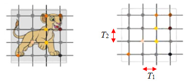
Fig.7 The 2D sampled image

If I find the spectrum of the sampled image shows above, it looks like Fig.8. It's not surprising this periodic because we do know  the spectrum of a discrete signal is periodic a property that we covered in quite some detail. And it is formed really by performing the periodic extension of the spectrum of the analog signal.(in section 2.(5)，Fourier transform of the sampled function is a infinite, periodic sequence of copies of  F(μ).)

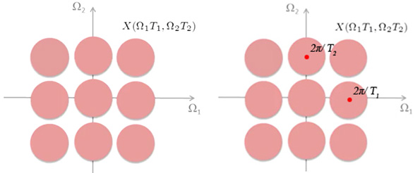
Fig.8 The spectrum of the sampled image

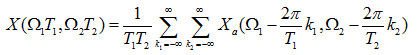
The mathematical expression to describe this, is the one shown here

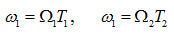
So far we've been using this notation ω₁, ω₂ denote the Fourier Transform of a discreet signal, and ω₁ is the normalized frequency and ω₁=Ω₁T₁. So ω₁is in rads(unit), while Ω₁is in rads per unit spatial distance (for example: rads/mm).

So what this expression tells me again is that they take the spectrum of the analog signal, and I periodically extend it. So k₁ ranges from (-∞,+∞), and so does k₂. And the periodic extension in the horizontal direction is with respect to 2π/ T₁ . The vertical direction with respect to 2π/ T₂. So the red point in Fig.8 is 2π/ T₁ and 2π/ T₂, respectively.

We see that in performing sampling, there are two important parameters: the sampling periods,  T₁, T₂. They  control the  spacing of the point in the spatial domain, and they also  control how far apart the replicas of the analog spectrum in this periodic extension, are going to be located.

(3) 2D critical-sampled

We say that the analog image is critical sampled, if I use the appropriate sampling period T₁, T₂ here. So that when I find now the Fourier transform of a discrete signal, which is formed by the periodic extension of the spectrum of the analog signal, the spectra here just touch, next to each other without overlapping. And in this case, at least mathematically speaking, I can filter the base band of the spectrum of the discrete signal, and then this will give me back the spectrum of the analog signal, therefore, I will be able to go from the discrete world, back to the continuous world without losing any information.

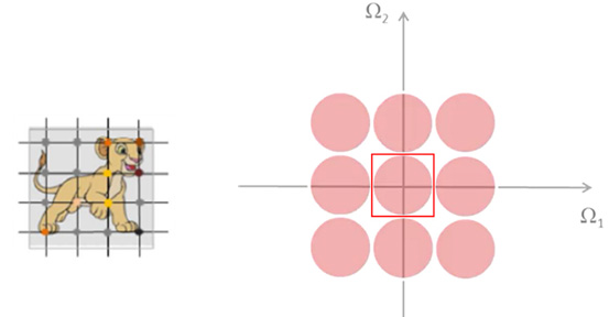
Fig.9 Critical-sampled image and its spectrum

(4) 2D over-sampled

If I use a smaller T₁,T₂ sampling periods than in the previous case, then when I look at the spectrum of the discrete signal, isgoing to look like Fig.10. And, in this case I've used more samples I needed to represent accurately the continuous image. Therefore, I have over-sampled.

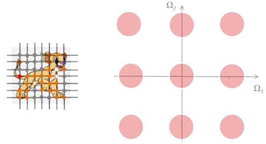
Fig.10 Over-sampled image and its spectrum

(5) 2D down-sampled

If I go the other direction, and use sampling periods here T₁,T₂, which are greater than the periods used for critical sampling. Then the spectrum of the discrete image, it looks like Fig.11(b), with new periodic extension, one replica over laps with another replica, and this phenomenon is referred to as aliasing. Which means that the high frequencies here alias themselves as low frequencies. Under this case, it's not possible to recover the original signal. I am not able to untangle the low and high frequencies that can be, mixed up.

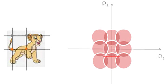
Fig.11 Down-sampledimage and its spectrum

(6) 2D Nyquist Theorem

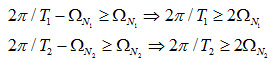
In performing sampling, an important questionis what should the samplings periods T₁,T₂ be equaled to? So that, I'm able to go back from the discrete samples to the analog image. Intuitively, one should expect that how close together the samples are should be a function of the spatial frequency in an image. If the image intensity varies a lot and rapidly, which means that there's a lot ofhigh-frequency energy. Then, intuitively, one should use samples that are close together, so that all of these first variations of intensity have captured the property. If on the other hand, they have another flat image, then a few samples will suffice, and this is exactly what the Nyquist theorem tells us. Fig.12 is again the support of the spectrum of the analog image, and lets callΩ_N1 the highest frequency in the horizontal direction and Ω_N2 the highest frequency in the vertical direction. After I sample this image, assume the spectrum of the discrete image looks like Fig.12. So in other words, there is no aliasing.

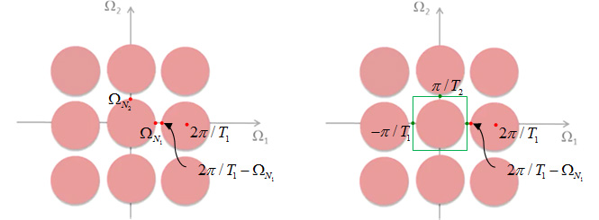
Fig.12 2D sampled image and its spectrum                       Fig.13 Low pass filter in the frequency domain

As long as  2π/T₁ -Ω_N1≥Ω_N1 , there's no aliasing in the horizontal direction. And this gives us the condition that  the sampling frequency should be at least twice as high as the highest frequency in the image. And they can obtain the similar condition in the vertical direction, so the sampling frequency in the vertical direction should be greater equal then  Ω_N1. 

So if these two conditions are satisfied, then I can recover the analog image from the discrete one by using a low pass filter (the green rectangle), as shown in Fig.13. The low pass filter can be written as:

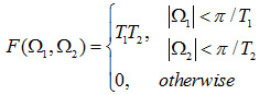
This T₁T₂ gain is here because of that, at the relationship between the spectrum of the discrete signal and the analog signal, there's 1/ T₁T₂ factor there. So I need this gain to bring back the signal its original values.

In summary what the Nyquist Theorem is telling me is that if I have an unlimited analog signal I can sample it with frequencies that satisfies these conditions. And then I can recover the analog signal from the discrete one using a filter like this on the frequency domain.