torch.nn 到底是什么？

What is torch.nn really?

Authors: Jeremy Howard, fast.ai. Thanks to Rachel Thomas and Francisco Ingham.

We recommend running this tutorial as a notebook, not a script. To download the notebook (.ipynb) file, click the link at the top of the page.

PyTorch provides the elegantly designed modules and classes torch.nn , torch.optim , Dataset , and DataLoader to help you create and train neural networks. In order to fully utilize their power and customize them for your problem, you need to really understand exactly what they’re doing. To develop this understanding, we will first train basic neural net on the MNIST data set without using any features from these models; we will initially only use the most basic PyTorch tensor functionality. Then, we will incrementally add one feature from torch.nn, torch.optim, Dataset, or DataLoader at a time, showing exactly what each piece does, and how it works to make the code either more concise, or more flexible.

This tutorial assumes you already have PyTorch installed, and are familiar with the basics of tensor operations. (If you’re familiar with Numpy array operations, you’ll find the PyTorch tensor operations used here nearly identical).

我们建议将本教程作为notebook而非脚本运行。要下载notebook (.ipynb) 文件，请单击页面顶部的链接。

PyTorch 提供了设计优雅的模块和类 torch.nn 、torch.optim 、Dataset 和 DataLoader，以帮助您创建和训练神经网络。为了充分利用它们的强大功能，并针对您的问题对它们进行定制，您需要真正理解它们到底在做什么。为了加深这种理解，我们将首先在 MNIST 数据集上训练基本的神经网络，但不使用这些模型中的任何特征；我们最初将只使用最基本的 PyTorch 张量功能。然后，我们将每次从 torch.nn、torch.optim、Dataset 或 DataLoader 中逐步添加一个特征，展示每个特征的确切作用，以及它是如何使代码更简洁或更灵活的。

本教程假定你已经安装了 PyTorch，并且熟悉张量运算的基础知识。(如果你熟悉 Numpy 数组操作，你会发现这里使用的 PyTorch 张量运算几乎相同）。

MNIST data setup

We will use the classic MNIST dataset, which consists of black-and-white images of hand-drawn digits (between 0 and 9).

We will use pathlib for dealing with paths (part of the Python 3 standard library), and will download the dataset using requests. We will only import modules when we use them, so you can see exactly what’s being used at each point.

我们将使用经典的 MNIST 数据集，该数据集由手绘数字（0 到 9 之间）的黑白图像组成。

我们将使用 pathlib 处理路径（Python 3 标准库的一部分），并使用requests下载数据集。我们只会在使用模块时才导入它们，这样你就能清楚地看到每一点都用到了什么。

from pathlib import Path
import requests

DATA_PATH = Path("data")
PATH = DATA_PATH / "mnist"

PATH.mkdir(parents=True, exist_ok=True)

URL = "https://github.com/pytorch/tutorials/raw/main/_static/"
FILENAME = "mnist.pkl.gz"

if not (PATH / FILENAME).exists():
        content = requests.get(URL + FILENAME).content
        (PATH / FILENAME).open("wb").write(content)

This dataset is in numpy array format, and has been stored using pickle, a python-specific format for serializing data.

该数据集采用 numpy 数组格式，并使用 Python 专用的数据序列化格式 pickle 进行存储。

import pickle
import gzip

with gzip.open((PATH / FILENAME).as_posix(), "rb") as f:
        ((x_train, y_train), (x_valid, y_valid), _) = pickle.load(f, encoding="latin-1")

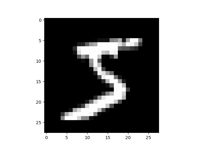
Each image is 28 x 28, and is being stored as a flattened row of length 784 (=28x28). Let’s take a look at one; we need to reshape it to 2d first.

每幅图像的大小为 28 x 28，以长度为 784（=28x28）的扁平行存储。让我们来看看其中一幅；我们需要先将其重塑为 2d 格式。

from matplotlib import pyplot
import numpy as np

pyplot.imshow(x_train[0].reshape((28, 28)), cmap="gray")
# ``pyplot.show()`` only if not on Colab
try:
    import google.colab
except ImportError:
    pyplot.show()
print(x_train.shape)

(50000, 784)

PyTorch uses torch.tensor, rather than numpy arrays, so we need to convert our data.

PyTorch 使用 torch.tensor，而不是 numpy 数组，因此我们需要转换数据。

import torch

x_train, y_train, x_valid, y_valid = map(
    torch.tensor, (x_train, y_train, x_valid, y_valid)
)
n, c = x_train.shape
print(x_train, y_train)
print(x_train.shape)
print(y_train.min(), y_train.max())

tensor([[0., 0., 0.,  ..., 0., 0., 0.],
        [0., 0., 0.,  ..., 0., 0., 0.],
        [0., 0., 0.,  ..., 0., 0., 0.],
        ...,
        [0., 0., 0.,  ..., 0., 0., 0.],
        [0., 0., 0.,  ..., 0., 0., 0.],
        [0., 0., 0.,  ..., 0., 0., 0.]]) tensor([5, 0, 4,  ..., 8, 4, 8])
torch.Size([50000, 784])
tensor(0) tensor(9)

Neural net from scratch (without torch.nn)

Let’s first create a model using nothing but PyTorch tensor operations. We’re assuming you’re already familiar with the basics of neural networks. (If you’re not, you can learn them at course.fast.ai).

PyTorch provides methods to create random or zero-filled tensors, which we will use to create our weights and bias for a simple linear model. These are just regular tensors, with one very special addition: we tell PyTorch that they require a gradient. This causes PyTorch to record all of the operations done on the tensor, so that it can calculate the gradient during back-propagation automatically!

For the weights, we set requires_grad after the initialization, since we don’t want that step included in the gradient. (Note that a trailing _ in PyTorch signifies that the operation is performed in-place.)

让我们先用 PyTorch 张量运算创建一个模型。我们假设您已经熟悉神经网络的基础知识。(如果还不熟悉，可以在 course.fast.ai 上学习）。

PyTorch 提供了创建随机或零填充张量的方法，我们将用它来为一个简单的线性模型创建权重和偏置。这些只是普通的张量，但有一个非常特殊的附加条件：我们告诉 PyTorch 它们需要梯度。这将导致 PyTorch 记录对张量进行的所有操作，以便在反向传播过程中自动计算梯度！

对于权重，我们在初始化后设置 requirements_grad，因为我们不希望将这一步包含在梯度中。(注意，在 PyTorch 中，尾部的 _ 表示操作是原地执行的）。

NOTE

We are initializing the weights here with Xavier initialisation (by multiplying with 1/sqrt(n)).

在这里，我们使用 Xavier 初始化法对权重进行初始化（乘以 1/sqrt(n)）。

import math

weights = torch.randn(784, 10) / math.sqrt(784)
weights.requires_grad_()
bias = torch.zeros(10, requires_grad=True)

Thanks to PyTorch’s ability to calculate gradients automatically, we can use any standard Python function (or callable object) as a model! So let’s just write a plain matrix multiplication and broadcasted addition to create a simple linear model. We also need an activation function, so we’ll write log_softmax and use it. Remember: although PyTorch provides lots of prewritten loss functions, activation functions, and so forth, you can easily write your own using plain python. PyTorch will even create fast GPU or vectorized CPU code for your function automatically.

由于 PyTorch 能够自动计算梯度，我们可以使用任何标准 Python 函数（或可调用对象）作为模型！因此，我们只需编写一个普通的矩阵乘法和广播加法，就能创建一个简单的线性模型。我们还需要一个激活函数，所以我们要写 log_softmax 并使用它。记住：尽管 PyTorch 提供了很多预写的损失函数、激活函数等，但你也可以用普通的 python 轻松地编写自己的函数。PyTorch 甚至会自动为你的函数创建快速的 GPU 或矢量化 CPU 代码。

def log_softmax(x):
    return x - x.exp().sum(-1).log().unsqueeze(-1)

def model(xb):
    return log_softmax(xb @ weights + bias)

In the above, the @ stands for the matrix multiplication operation. We will call our function on one batch of data (in this case, 64 images). This is one forward pass. Note that our predictions won’t be any better than random at this stage, since we start with random weights.

在上文中，@ 代表矩阵乘法运算。我们将对一批数据（本例中为 64 幅图像）调用我们的函数。这是一次前向传递。请注意，在这一阶段，我们的预测结果不会比随机结果更好，因为我们一开始使用的是随机权重。

bs = 64  # batch size

xb = x_train[0:bs]  # a mini-batch from x
preds = model(xb)  # predictions
preds[0], preds.shape
print(preds[0], preds.shape)

tensor([-2.5452, -2.0790, -2.1832, -2.6221, -2.3670, -2.3854, -2.9432, -2.4391,
        -1.8657, -2.0355], grad_fn=<SelectBackward0>) torch.Size([64, 10])

As you see, the preds tensor contains not only the tensor values, but also a gradient function. We’ll use this later to do backprop.

Let’s implement negative log-likelihood to use as the loss function (again, we can just use standard Python):

如您所见，preds 张量不仅包含张量值，还包含一个梯度函数。我们稍后将用它来进行反推。

让我们实现负对数似然作为损失函数（同样，我们可以直接使用标准 Python）：

def nll(input, target):
    return -input[range(target.shape[0]), target].mean()

loss_func = nll

Let’s check our loss with our random model, so we can see if we improve after a backprop pass later.

让我们用随机模型检查一下损失，这样我们就能知道在之后的反向推演中是否有所改进。

yb = y_train[0:bs]
print(loss_func(preds, yb))

tensor(2.4020, grad_fn=<NegBackward0>)

Let’s also implement a function to calculate the accuracy of our model. For each prediction, if the index with the largest value matches the target value, then the prediction was correct.

我们还要实现一个函数来计算模型的准确性。对于每次预测，如果最大值的索引与目标值相匹配，那么预测就是正确的。

def accuracy(out, yb):
    preds = torch.argmax(out, dim=1)
    return (preds == yb).float().mean()

Let’s check the accuracy of our random model, so we can see if our accuracy improves as our loss improves.

让我们检查一下随机模型的准确性，看看我们的准确性是否会随着损失的增加而提高。

print(accuracy(preds, yb))

tensor(0.0938)

We can now run a training loop. For each iteration, we will:

• select a mini-batch of data (of size bs)
• use the model to make predictions
• calculate the loss
• loss.backward() updates the gradients of the model, in this case, weights and bias.

We now use these gradients to update the weights and bias. We do this within the torch.no_grad() context manager, because we do not want these actions to be recorded for our next calculation of the gradient. You can read more about how PyTorch’s Autograd records operations here.

We then set the gradients to zero, so that we are ready for the next loop. Otherwise, our gradients would record a running tally of all the operations that had happened (i.e. loss.backward() adds the gradients to whatever is already stored, rather than replacing them).

现在我们可以运行一个训练循环。每次迭代时，我们将

• 选择一批小型数据（大小为 bs）

• 使用模型进行预测

• 计算损失

• loss.backward() 更新模型的梯度，本例中为权重和偏差。

现在我们使用这些梯度来更新权重和偏置。我们是在 torch.no_grad() 上下文管理器中完成这一操作的，因为我们不希望在下一次计算梯度时记录这些操作。有关 PyTorch 的 Autograd 如何记录操作的更多信息，请点击此处。

然后，我们将梯度设置为零，以便为下一个循环做好准备。否则，我们的梯度将记录下所有操作的流水账（即 loss.backward() 将梯度添加到已存储的操作中，而不是替换它们）。

TIP

You can use the standard python debugger to step through PyTorch code, allowing you to check the various variable values at each step. Uncomment set_trace() below to try it out.

你可以使用标准的 python 调试器来步进 PyTorch 代码，这样你就可以检查每一步的各种变量值。请取消下面的 set_trace() 来尝试一下。

from IPython.core.debugger import set_trace

lr = 0.5  # learning rate
epochs = 2  # how many epochs to train for

for epoch in range(epochs):
    for i in range((n - 1) // bs + 1):
        #         set_trace()
        start_i = i * bs
        end_i = start_i + bs
        xb = x_train[start_i:end_i]
        yb = y_train[start_i:end_i]
        pred = model(xb)
        loss = loss_func(pred, yb)

        loss.backward()
        with torch.no_grad():
            weights -= weights.grad * lr
            bias -= bias.grad * lr
            weights.grad.zero_()
            bias.grad.zero_()

That’s it: we’ve created and trained a minimal neural network (in this case, a logistic regression, since we have no hidden layers) entirely from scratch!

Let’s check the loss and accuracy and compare those to what we got earlier. We expect that the loss will have decreased and accuracy to have increased, and they have.

就是这样：我们完全从零开始创建并训练了一个最小的神经网络（在本例中是逻辑回归，因为我们没有隐藏层）！

让我们检查一下损失和准确率，并与之前的结果进行比较。我们预计损失会减少，准确率会提高，结果确实如此。

print(loss_func(model(xb), yb), accuracy(model(xb), yb))

tensor(0.0813, grad_fn=<NegBackward0>) tensor(1.)

Using torch.nn.functional

We will now refactor our code, so that it does the same thing as before, only we’ll start taking advantage of PyTorch’s nn classes to make it more concise and flexible. At each step from here, we should be making our code one or more of: shorter, more understandable, and/or more flexible.

The first and easiest step is to make our code shorter by replacing our hand-written activation and loss functions with those from torch.nn.functional (which is generally imported into the namespace F by convention). This module contains all the functions in the torch.nn library (whereas other parts of the library contain classes). As well as a wide range of loss and activation functions, you’ll also find here some convenient functions for creating neural nets, such as pooling functions. (There are also functions for doing convolutions, linear layers, etc, but as we’ll see, these are usually better handled using other parts of the library.)

If you’re using negative log likelihood loss and log softmax activation, then Pytorch provides a single function F.cross_entropy that combines the two. So we can even remove the activation function from our model.

现在我们将重构我们的代码，使其做与之前相同的事情，只是我们将开始利用 PyTorch 的 nn 类，使其更加简洁和灵活。从现在起，每一步我们都要使代码在变得更简短、更易懂和/或更灵活。

第一步，也是最简单的一步，就是用 torch.nn.functional 中的函数（按照惯例，通常导入到命名空间 F 中）取代我们手写的激活和损失函数，从而缩短我们的代码。该模块包含 torch.nn 库中的所有函数（而库的其他部分包含类）。除了大量的损失和激活函数外，你还能在这里找到一些用于创建神经网络的便捷函数，例如池化函数。(也有用于卷积、线性层等的函数，但正如我们将看到的，这些函数通常使用库的其他部分处理效果更好）。

如果你使用的是 negative log likelihood loss 和 log softmax activation ，那么 Pytorch 会提供一个函数 F.cross_entropy，将两者结合起来。因此，我们甚至可以从模型中移除激活函数。

import torch.nn.functional as F

loss_func = F.cross_entropy

def model(xb):
    return xb @ weights + bias

Note that we no longer call log_softmax in the model function. Let’s confirm that our loss and accuracy are the same as before:

请注意，我们不再在 model 函数中调用 log_softmax。让我们确认一下损失和准确率是否与之前相同：

print(loss_func(model(xb), yb), accuracy(model(xb), yb))

tensor(0.0813, grad_fn=<NllLossBackward0>) tensor(1.)

Refactor using nn.Module

Next up, we’ll use nn.Module and nn.Parameter, for a clearer and more concise training loop. We subclass nn.Module (which itself is a class and able to keep track of state). In this case, we want to create a class that holds our weights, bias, and method for the forward step. nn.Module has a number of attributes and methods (such as .parameters() and .zero_grad()) which we will be using.

接下来，我们将使用 nn.Module 和 nn.Parameter，使训练循环更加清晰简洁。我们子类化 nn.Module（它本身是一个类，能够跟踪状态）。在本例中，我们要创建一个类，用于保存权重、偏置和前进步骤的方法。nn.Module 有许多属性和方法（如 .parameters() 和 .zero_grad()），我们将使用这些属性和方法。

NOTE

nn.Module (uppercase M) is a PyTorch specific concept, and is a class we’ll be using a lot. nn.Module is not to be confused with the Python concept of a (lowercase m) module, which is a file of Python code that can be imported.

nn.Module（大写 M）是 PyTorch 特有的概念，也是我们会经常用到的一个类。nn.Module 不能与 Python 的module（小写 m）概念混淆，后者是一个可以导入的 Python 代码文件。

from torch import nn

class Mnist_Logistic(nn.Module):
    def __init__(self):
        super().__init__()
        self.weights = nn.Parameter(torch.randn(784, 10) / math.sqrt(784))
        self.bias = nn.Parameter(torch.zeros(10))

    def forward(self, xb):
        return xb @ self.weights + self.bias

Since we’re now using an object instead of just using a function, we first have to instantiate our model:

由于我们现在使用的是一个对象，而不仅仅是一个函数，所以我们首先要实例化我们的模型：

model = Mnist_Logistic()

Now we can calculate the loss in the same way as before. Note that nn.Module objects are used as if they are functions (i.e they are callable), but behind the scenes Pytorch will call our forward method automatically.

现在，我们可以像以前一样计算损失。请注意，nn.Module 对象被当作函数使用（即它们是可调用的），但在幕后 Pytorch 会自动调用我们的 forward 方法。

print(loss_func(model(xb), yb))

tensor(2.3096, grad_fn=<NllLossBackward0>)

Previously for our training loop we had to update the values for each parameter by name, and manually zero out the grads for each parameter separately, like this:

以前，在训练循环中，我们必须按名称更新每个参数的值，并分别手动清零每个参数的粒度，就像这样：

with torch.no_grad():
    weights -= weights.grad * lr
    bias -= bias.grad * lr
    weights.grad.zero_()
    bias.grad.zero_()

Now we can take advantage of model.parameters() and model.zero_grad() (which are both defined by PyTorch for nn.Module) to make those steps more concise and less prone to the error of forgetting some of our parameters, particularly if we had a more complicated model:

现在，我们可以利用 model.parameters() 和 model.zero_grad()（这两个参数都是 PyTorch 为 nn.Module 定义的），使这些步骤更加简洁，不容易忘记某些参数，尤其是当我们有一个更复杂的模型时：

with torch.no_grad():
    for p in model.parameters(): p -= p.grad * lr
    model.zero_grad()

We’ll wrap our little training loop in a fit function so we can run it again later.

我们将用一个 fit 函数来封装我们的训练小循环，以便以后再次运行。

def fit():
    for epoch in range(epochs):
        for i in range((n - 1) // bs + 1):
            start_i = i * bs
            end_i = start_i + bs
            xb = x_train[start_i:end_i]
            yb = y_train[start_i:end_i]
            pred = model(xb)
            loss = loss_func(pred, yb)

            loss.backward()
            with torch.no_grad():
                for p in model.parameters():
                    p -= p.grad * lr
                model.zero_grad()

fit()

Let’s double-check that our loss has gone down:

让我们再确认一下，我们的损失是否已经减少：

print(loss_func(model(xb), yb))

tensor(0.0821, grad_fn=<NllLossBackward0>)

Refactor using nn.Linear

We continue to refactor our code. Instead of manually defining and initializing self.weights and self.bias, and calculating xb @ self.weights + self.bias, we will instead use the Pytorch class nn.Linear for a linear layer, which does all that for us. Pytorch has many types of predefined layers that can greatly simplify our code, and often makes it faster too.

我们将继续重构代码。我们不需要手动定义和初始化 self.weights 和 self.bias，也不需要计算 xb @ self.weights + self.bias，而是使用 Pytorch 类 nn.Linear 作为线性层，它可以为我们完成所有这些工作。Pytorch 有许多类型的预定义层，可以大大简化我们的代码，而且通常也会更快。

class Mnist_Logistic(nn.Module):
    def __init__(self):
        super().__init__()
        self.lin = nn.Linear(784, 10)

    def forward(self, xb):
        return self.lin(xb)

We instantiate our model and calculate the loss in the same way as before:

我们将模型实例化，并以与之前相同的方式计算损失：

model = Mnist_Logistic()
print(loss_func(model(xb), yb))

tensor(2.3313, grad_fn=<NllLossBackward0>)

We are still able to use our same fit method as before.

我们仍然可以使用与以前相同的 fit 方法。

fit()

print(loss_func(model(xb), yb))

tensor(0.0819, grad_fn=<NllLossBackward0>)

Refactor using torch.optim

Pytorch also has a package with various optimization algorithms, torch.optim. We can use the step method from our optimizer to take a forward step, instead of manually updating each parameter.

This will let us replace our previous manually coded optimization step:

Pytorch 还有一个包含各种优化算法的软件包 torch.optim。我们可以使用优化器中的 step 方法向前迈一步，而不用手动更新每个参数。

这将让我们取代之前手动编码的优化步骤：

with torch.no_grad():
    for p in model.parameters(): p -= p.grad * lr
    model.zero_grad()

and instead use just:

而只使用

opt.step()
opt.zero_grad()

(optim.zero_grad() resets the gradient to 0 and we need to call it before computing the gradient for the next minibatch.)

(optim.zero_grad()会将梯度重置为 0，我们需要在计算下一个迷你批次的梯度之前调用它）。

from torch import optim

We’ll define a little function to create our model and optimizer so we can reuse it in the future.

我们将定义一个小函数来创建模型和优化器，以便将来重复使用。

def get_model():
    model = Mnist_Logistic()
    return model, optim.SGD(model.parameters(), lr=lr)

model, opt = get_model()
print(loss_func(model(xb), yb))

for epoch in range(epochs):
    for i in range((n - 1) // bs + 1):
        start_i = i * bs
        end_i = start_i + bs
        xb = x_train[start_i:end_i]
        yb = y_train[start_i:end_i]
        pred = model(xb)
        loss = loss_func(pred, yb)

        loss.backward()
        opt.step()
        opt.zero_grad()

print(loss_func(model(xb), yb))

tensor(2.2659, grad_fn=<NllLossBackward0>)
tensor(0.0810, grad_fn=<NllLossBackward0>)

Refactor using Dataset

PyTorch has an abstract Dataset class. A Dataset can be anything that has a __len__ function (called by Python’s standard len function) and a __getitem__ function as a way of indexing into it. This tutorial walks through a nice example of creating a custom FacialLandmarkDataset class as a subclass of Dataset.

PyTorch’s TensorDataset is a Dataset wrapping tensors. By defining a length and way of indexing, this also gives us a way to iterate, index, and slice along the first dimension of a tensor. This will make it easier to access both the independent and dependent variables in the same line as we train.

PyTorch 有一个抽象的 Dataset 类。Dataset 可以是任何具有 __len__ 函数（由 Python 的标准 len 函数调用）和 __getitem__ 函数作为索引方式的东西。本教程将通过一个很好的示例来介绍如何创建一个自定义的 FacialLandmarkDataset 类作为 Dataset 的子类。

PyTorch 的 TensorDataset 是一个包裹张量的 Dataset。通过定义长度和索引方式，这也为我们提供了沿着张量的第一个维度进行迭代、索引和切片的方法。这将使我们在训练时更容易在同一行中访问自变量和因变量。

from torch.utils.data import TensorDataset

Both x_train and y_train can be combined in a single TensorDataset, which will be easier to iterate over and slice.

x_train 和 y_train 可以合并为一个 TensorDataset，这样就更容易遍历和切分。

train_ds = TensorDataset(x_train, y_train)

Previously, we had to iterate through minibatches of x and y values separately:

以前，我们必须分别遍历 x 和 y 值的迷你批次：

xb = x_train[start_i:end_i]
yb = y_train[start_i:end_i]

Now, we can do these two steps together:

现在，我们可以一起完成这两个步骤：

xb,yb = train_ds[i*bs : i*bs+bs]

model, opt = get_model()

for epoch in range(epochs):
    for i in range((n - 1) // bs + 1):
        xb, yb = train_ds[i * bs: i * bs + bs]
        pred = model(xb)
        loss = loss_func(pred, yb)

        loss.backward()
        opt.step()
        opt.zero_grad()

print(loss_func(model(xb), yb))

tensor(0.0826, grad_fn=<NllLossBackward0>)

Refactor using DataLoader

PyTorch’s DataLoader is responsible for managing batches. You can create a DataLoader from any Dataset. DataLoader makes it easier to iterate over batches. Rather than having to use train_ds[i*bs : i*bs+bs], the DataLoader gives us each minibatch automatically.

PyTorch 的 DataLoader 负责管理批次。你可以从任何 Dataset 创建一个 DataLoader。DataLoader 使批次迭代变得更容易。与使用 train_ds[i*bs：i*bs+bs]相比，DataLoader 会自动为我们提供每个小批量。

from torch.utils.data import DataLoader

train_ds = TensorDataset(x_train, y_train)
train_dl = DataLoader(train_ds, batch_size=bs)

Previously, our loop iterated over batches (xb, yb) like this:

之前，我们的循环是这样遍历批次 (xb, yb)的：

for i in range((n-1)//bs + 1):
    xb,yb = train_ds[i*bs : i*bs+bs]
    pred = model(xb)

Now, our loop is much cleaner, as (xb, yb) are loaded automatically from the data loader:

现在，我们的循环更简洁了，因为 (xb, yb) 会自动从数据加载器加载：

for xb,yb in train_dl:
    pred = model(xb)

model, opt = get_model()

for epoch in range(epochs):
    for xb, yb in train_dl:
        pred = model(xb)
        loss = loss_func(pred, yb)

        loss.backward()
        opt.step()
        opt.zero_grad()

print(loss_func(model(xb), yb))

tensor(0.0818, grad_fn=<NllLossBackward0>)

Thanks to PyTorch’s nn.Module, nn.Parameter, Dataset, and DataLoader, our training loop is now dramatically smaller and easier to understand. Let’s now try to add the basic features necessary to create effective models in practice.

多亏了 PyTorch 的 nn.Module、nn.Parameter、Dataset 和 DataLoader，我们的训练循环现在大大缩小了，也更容易理解了。现在，让我们尝试添加在实践中创建有效模型所需的基本功能。

Add validation

In section 1, we were just trying to get a reasonable training loop set up for use on our training data. In reality, you always should also have a validation set, in order to identify if you are overfitting.

Shuffling the training data is important to prevent correlation between batches and overfitting. On the other hand, the validation loss will be identical whether we shuffle the validation set or not. Since shuffling takes extra time, it makes no sense to shuffle the validation data.

We’ll use a batch size for the validation set that is twice as large as that for the training set. This is because the validation set does not need backpropagation and thus takes less memory (it doesn’t need to store the gradients). We take advantage of this to use a larger batch size and compute the loss more quickly.

在第 1 部分中，我们只是试图在训练数据上建立一个合理的训练循环。实际上，你还应该有一个验证集，以便识别是否过度拟合。

对训练数据进行打乱对于防止批次间的相关性和过度拟合非常重要。另一方面，无论我们是否打乱验证集，验证损失都是相同的。由于打乱需要额外的时间，因此打乱验证数据毫无意义。

我们将验证集的批次大小设定为训练集的两倍。这是因为验证集不需要反向传播，因此占用内存较少（不需要存储梯度）。我们利用这一优势，使用更大的批次规模，更快地计算损失。

train_ds = TensorDataset(x_train, y_train)
train_dl = DataLoader(train_ds, batch_size=bs, shuffle=True)

valid_ds = TensorDataset(x_valid, y_valid)
valid_dl = DataLoader(valid_ds, batch_size=bs * 2)

We will calculate and print the validation loss at the end of each epoch.

(Note that we always call model.train() before training, and model.eval() before inference, because these are used by layers such as nn.BatchNorm2d and nn.Dropout to ensure appropriate behavior for these different phases.)

我们将在每轮结束时计算并打印验证损失。

(请注意，我们总是在训练之前调用 model.train()，在推理之前调用 model.eval()，因为 nn.BatchNorm2d 和 nn.Dropout 等层会使用这些函数来确保这些不同阶段的适当行为）。

model, opt = get_model()

for epoch in range(epochs):
    model.train()
    for xb, yb in train_dl:
        pred = model(xb)
        loss = loss_func(pred, yb)

        loss.backward()
        opt.step()
        opt.zero_grad()

    model.eval()
    with torch.no_grad():
        valid_loss = sum(loss_func(model(xb), yb) for xb, yb in valid_dl)

    print(epoch, valid_loss / len(valid_dl))

0 tensor(0.3048)
1 tensor(0.2872)

Create fit() and get_data()

We’ll now do a little refactoring of our own. Since we go through a similar process twice of calculating the loss for both the training set and the validation set, let’s make that into its own function, loss_batch, which computes the loss for one batch.

We pass an optimizer in for the training set, and use it to perform backprop. For the validation set, we don’t pass an optimizer, so the method doesn’t perform backprop.

现在，我们将对自己的函数进行一点重构。由于我们要经历两次计算训练集和验证集损失的类似过程，因此让我们把它变成自己的函数 loss_batch，用于计算一个批次的损失。

我们为训练集传递一个优化器，并用它来执行反推。对于验证集，我们不传递优化器，因此该方法不执行反推。

def loss_batch(model, loss_func, xb, yb, opt=None):
    loss = loss_func(model(xb), yb)

    if opt is not None:
        loss.backward()
        opt.step()
        opt.zero_grad()

    return loss.item(), len(xb)

fit runs the necessary operations to train our model and compute the training and validation losses for each epoch.

fit 运行必要的操作来训练我们的模型，并计算每轮的训练损失和验证损失。

import numpy as np

def fit(epochs, model, loss_func, opt, train_dl, valid_dl):
    for epoch in range(epochs):
        model.train()
        for xb, yb in train_dl:
            loss_batch(model, loss_func, xb, yb, opt)

        model.eval()
        with torch.no_grad():
            losses, nums = zip(
                *[loss_batch(model, loss_func, xb, yb) for xb, yb in valid_dl]
            )
        val_loss = np.sum(np.multiply(losses, nums)) / np.sum(nums)

        print(epoch, val_loss)

get_data returns dataloaders for the training and validation sets.

get_data 返回训练集和验证集的数据载体。

def get_data(train_ds, valid_ds, bs):
    return (
        DataLoader(train_ds, batch_size=bs, shuffle=True),
        DataLoader(valid_ds, batch_size=bs * 2),
    )

Now, our whole process of obtaining the data loaders and fitting the model can be run in 3 lines of code:

现在，我们获取数据加载器和拟合模型的整个过程只需 3 行代码即可完成：

train_dl, valid_dl = get_data(train_ds, valid_ds, bs)
model, opt = get_model()
fit(epochs, model, loss_func, opt, train_dl, valid_dl)

0 0.2939354367017746
1 0.3258970756947994

You can use these basic 3 lines of code to train a wide variety of models. Let’s see if we can use them to train a convolutional neural network (CNN)!

您可以使用这 3 行基本代码来训练各种模型。让我们看看能否用它们来训练一个卷积神经网络（CNN）！

Switch to CNN

We are now going to build our neural network with three convolutional layers. Because none of the functions in the previous section assume anything about the model form, we’ll be able to use them to train a CNN without any modification.

We will use PyTorch’s predefined Conv2d class as our convolutional layer. We define a CNN with 3 convolutional layers. Each convolution is followed by a ReLU. At the end, we perform an average pooling. (Note that view is PyTorch’s version of Numpy’s reshape)

现在，我们将用三个卷积层构建神经网络。由于上一节中的函数都不假定模型的任何形式，因此我们可以使用它们来训练 CNN，而无需做任何修改。

我们将使用 PyTorch 预定义的 Conv2d 类作为卷积层。我们定义了一个包含 3 个卷积层的 CNN。每个卷积层之后都有一个 ReLU。最后，我们进行平均池化。(请注意，view 是 PyTorch 版本的 Numpy reshape）。

class Mnist_CNN(nn.Module):
    def __init__(self):
        super().__init__()
        self.conv1 = nn.Conv2d(1, 16, kernel_size=3, stride=2, padding=1)
        self.conv2 = nn.Conv2d(16, 16, kernel_size=3, stride=2, padding=1)
        self.conv3 = nn.Conv2d(16, 10, kernel_size=3, stride=2, padding=1)

    def forward(self, xb):
        xb = xb.view(-1, 1, 28, 28)
        xb = F.relu(self.conv1(xb))
        xb = F.relu(self.conv2(xb))
        xb = F.relu(self.conv3(xb))
        xb = F.avg_pool2d(xb, 4)
        return xb.view(-1, xb.size(1))

lr = 0.1

Momentum is a variation on stochastic gradient descent that takes previous updates into account as well and generally leads to faster training.

动量法是随机梯度下降法的一种变体，它也考虑了之前的更新，通常能加快训练速度。

model = Mnist_CNN()
opt = optim.SGD(model.parameters(), lr=lr, momentum=0.9)

fit(epochs, model, loss_func, opt, train_dl, valid_dl)

0 0.35247018008232117
1 0.25782823679447175

Using nn.Sequential

torch.nn has another handy class we can use to simplify our code: Sequential . A Sequential object runs each of the modules contained within it, in a sequential manner. This is a simpler way of writing our neural network.

To take advantage of this, we need to be able to easily define a custom layer from a given function. For instance, PyTorch doesn’t have a view layer, and we need to create one for our network. Lambda will create a layer that we can then use when defining a network with Sequential.

torch.nn 还有一个方便的类，我们可以用它来简化代码： Sequential。一个 Sequential 对象可以按顺序运行其中包含的每个模块。这是编写神经网络的一种更简单的方法。

为了利用这一优势，我们需要能够轻松地从给定函数中定义自定义层。例如，PyTorch 没有视图层，我们需要为我们的网络创建一个视图层。Lambda 将创建一个层，然后我们就可以在使用 Sequential 定义网络时使用它。

class Lambda(nn.Module):
    def __init__(self, func):
        super().__init__()
        self.func = func

    def forward(self, x):
        return self.func(x)


def preprocess(x):
    return x.view(-1, 1, 28, 28)

The model created with Sequential is simple:

使用 Sequential 创建的模型非常简单：

model = nn.Sequential(
    Lambda(preprocess),
    nn.Conv2d(1, 16, kernel_size=3, stride=2, padding=1),
    nn.ReLU(),
    nn.Conv2d(16, 16, kernel_size=3, stride=2, padding=1),
    nn.ReLU(),
    nn.Conv2d(16, 10, kernel_size=3, stride=2, padding=1),
    nn.ReLU(),
    nn.AvgPool2d(4),
    Lambda(lambda x: x.view(x.size(0), -1)),
)

opt = optim.SGD(model.parameters(), lr=lr, momentum=0.9)

fit(epochs, model, loss_func, opt, train_dl, valid_dl)

0 0.3226209937572479
1 0.2234949318766594

Wrapping DataLoader

• Our CNN is fairly concise, but it only works with MNIST, because:

  It assumes the input is a 2828 long vectorIt assumes that the final CNN grid size is 44 (since that’s the average pooling kernel size we used)

Let’s get rid of these two assumptions, so our model works with any 2d single channel image. First, we can remove the initial Lambda layer by moving the data preprocessing into a generator:

我们的 CNN 相当简洁，但只适用于 MNIST，因为：

• 它假定输入是一个 28*28 的长向量
• 假设最终的 CNN 网格大小为 4*4（因为这是我们使用的平均池核大小）

让我们去掉这两个假设，这样我们的模型就能适用于任何 2d 单通道图像了。首先，我们可以将数据预处理移至生成器中，从而移除初始 Lambda 层：

def preprocess(x, y):
    return x.view(-1, 1, 28, 28), y


class WrappedDataLoader:
    def __init__(self, dl, func):
        self.dl = dl
        self.func = func

    def __len__(self):
        return len(self.dl)

    def __iter__(self):
        for b in self.dl:
            yield (self.func(*b))

train_dl, valid_dl = get_data(train_ds, valid_ds, bs)
train_dl = WrappedDataLoader(train_dl, preprocess)
valid_dl = WrappedDataLoader(valid_dl, preprocess)

Next, we can replace nn.AvgPool2d with nn.AdaptiveAvgPool2d, which allows us to define the size of the output tensor we want, rather than the input tensor we have. As a result, our model will work with any size input.

接下来，我们可以用 nn.AdaptiveAvgPool2d 代替 nn.AvgPool2d，这样就可以定义我们想要的输出张量的大小，而不是输入张量的大小。因此，我们的模型可以在任何大小的输入中运行。

model = nn.Sequential(
    nn.Conv2d(1, 16, kernel_size=3, stride=2, padding=1),
    nn.ReLU(),
    nn.Conv2d(16, 16, kernel_size=3, stride=2, padding=1),
    nn.ReLU(),
    nn.Conv2d(16, 10, kernel_size=3, stride=2, padding=1),
    nn.ReLU(),
    nn.AdaptiveAvgPool2d(1),
    Lambda(lambda x: x.view(x.size(0), -1)),
)

opt = optim.SGD(model.parameters(), lr=lr, momentum=0.9)

Let’s try it out:

让我们试一试：

fit(epochs, model, loss_func, opt, train_dl, valid_dl)

0 0.3148617018699646
1 0.20678156037330628

Using your GPU

If you’re lucky enough to have access to a CUDA-capable GPU (you can rent one for about $0.50/hour from most cloud providers) you can use it to speed up your code. First check that your GPU is working in Pytorch:

如果你有幸能使用支持 CUDA 的 GPU（你可以从大多数云提供商那里以大约 0.50 美元/小时的价格租用一个），你就可以用它来加速你的代码。首先在 Pytorch 中检查 GPU 是否正常工作：

print(torch.cuda.is_available())

True

And then create a device object for it:

然后为其创建一个设备对象：

dev = torch.device(
    "cuda") if torch.cuda.is_available() else torch.device("cpu")

Let’s update preprocess to move batches to the GPU:

让我们更新预处理，将批处理移至 GPU：

def preprocess(x, y):
    return x.view(-1, 1, 28, 28).to(dev), y.to(dev)


train_dl, valid_dl = get_data(train_ds, valid_ds, bs)
train_dl = WrappedDataLoader(train_dl, preprocess)
valid_dl = WrappedDataLoader(valid_dl, preprocess)

Finally, we can move our model to the GPU.

最后，我们可以将模型移动到 GPU 上。

model.to(dev)
opt = optim.SGD(model.parameters(), lr=lr, momentum=0.9)

You should find it runs faster now:

你会发现它现在运行得更快了：

fit(epochs, model, loss_func, opt, train_dl, valid_dl)

0 0.18022174834012986
1 0.17118794825077058

Closing thoughts

We now have a general data pipeline and training loop which you can use for training many types of models using Pytorch. To see how simple training a model can now be, take a look at the mnist_sample notebook.

Of course, there are many things you’ll want to add, such as data augmentation, hyperparameter tuning, monitoring training, transfer learning, and so forth. These features are available in the fastai library, which has been developed using the same design approach shown in this tutorial, providing a natural next step for practitioners looking to take their models further.

We promised at the start of this tutorial we’d explain through example each of torch.nn, torch.optim, Dataset, and DataLoader. So let’s summarize what we’ve seen:

我们现在有了一个通用的数据管道和训练循环，你可以用它来使用 Pytorch 训练多种类型的模型。要想知道训练模型有多简单，请看 mnist_sample notebook。

当然，你还想添加很多功能，比如数据增强、超参数调整、监控训练、迁移学习等等。fastai 库提供了这些功能，该库的开发采用了本教程中展示的相同设计方法，为希望进一步完善模型的实践者提供了一个自然的下一步。

在本教程的开头，我们承诺将通过示例逐一解释 torch.nn、torrent.optim、Dataset 和 DataLoader。下面让我们总结一下我们所看到的内容：

• torch.nn:
  • Module: creates a callable which behaves like a function, but can also contain state(such as neural net layer weights). It knows what Parameter (s) it contains and can zero all their gradients, loop through them for weight updates, etc.
  • Parameter: a wrapper for a tensor that tells a Module that it has weights that need updating during backprop. Only tensors with the requires_grad attribute set are updated
  • functional: a module(usually imported into the F namespace by convention) which contains activation functions, loss functions, etc, as well as non-stateful versions of layers such as convolutional and linear layers.
• torch.optim: Contains optimizers such as SGD, which update the weights of Parameter during the backward step
• Dataset: An abstract interface of objects with a __len__ and a __getitem__, including classes provided with Pytorch such as TensorDataset
• DataLoader: Takes any Dataset and creates an iterator which returns batches of data.
• torch.nn：
  • Module：创建一个可调用函数，其行为类似函数，但也可以包含状态（如神经网层权重）。它知道自己包含哪些 Parameter，并能将所有参数的梯度归零，循环使用这些参数进行权重更新等。
  • Parameter：张量的包装器，用于告诉 Module 它有需要在逆推过程中更新的权重。只有设置了 requires_grad 属性的张量才会被更新
  • functional：模块（通常按照惯例导入 F 命名空间），包含激活函数、损失函数等，以及卷积层和线性层等非状态化版本。
• torrent.optim：包含优化器（如 SGD），可在后退步骤中更新 Parameter 的权重
• Dataset：具有 __len__ 和 __getitem__ 的对象的抽象接口，包括 Pytorch 提供的类，如 TensorDataset
• DataLoader：接收任何 Dataset 并创建一个迭代器，返回成批的数据。

Total running time of the script: ( 0 minutes 35.142 seconds)