ComplexHeatmap热图专栏 | 6. 3D热图绘制教程

小杜的生信筆記

已于 2023-12-07 17:28:06 修改

阅读量816

点赞数 20

分类专栏： R语言精美图形绘制教程文章标签：数据库开发语言学习网络图热图 3D热图生物信息学

于 2023-12-07 17:24:41 首次发布

本文链接：https://blog.csdn.net/kanghua_du/article/details/134860739

版权

R语言精美图形绘制教程专栏收录该内容

82 篇文章 21 订阅

订阅专栏

本期教程

原文链接https://mp.weixin.qq.com/s/EyBs6jn78zOomcTv1aP52g

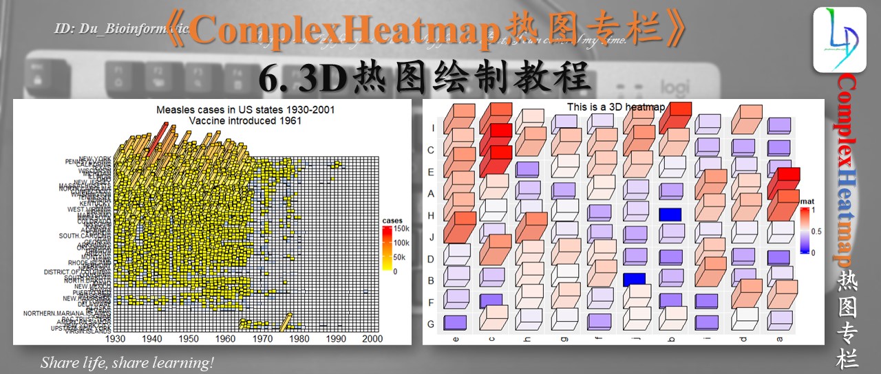
6 3D热图的绘制教程

基于《热图绘制教程》专栏，本教程已更新了5个章节，不知道大家是否有所收获。对于小杜个人来说，真的需要不断的复习和练习才可以记住，但是在自己使用的时候也需要重复的看自己的学习笔记。这就是“为什么需要我们不断地练习”的原因吧。

《热图绘制教程》专栏我们通说更新发哦《生信知识库》中，你可以到知识库中查看和学习。

6.1 安装和加载所需的包

library(ComplexHeatmap)

6.2 加载所需数据

set.seed(123)
mat = matrix(rnorm(500), ncol = 10)
colnames(mat) = letters[1:10]
head(mat)

  a           b           c          d          e           f          g          h           i          j
[1,] -0.56047565  0.25331851 -0.71040656  0.7877388  2.1988103 -0.37560287 -0.7152422  1.0149432 -0.07355602  1.4304023
[2,] -0.23017749 -0.02854676  0.25688371  0.7690422  1.3124130 -0.56187636 -0.7526890 -1.9927485 -1.16865142  1.0466288
[3,]  1.55870831 -0.04287046 -0.24669188  0.3322026 -0.2651451 -0.34391723 -0.9385387 -0.4272793 -0.63474826  0.4352889
[4,]  0.07050839  1.36860228 -0.34754260 -1.0083766  0.5431941  0.09049665 -1.0525133  0.1166373 -0.02884155  0.7151784
[5,]  0.12928774 -0.22577099 -0.95161857 -0.1194526 -0.4143399  1.59850877 -0.4371595 -0.8932076  0.67069597  0.9171749
[6,]  1.71506499  1.51647060 -0.04502772 -0.2803953 -0.4762469 -0.08856511  0.3311792  0.3339029 -1.65054654 -2.6609228

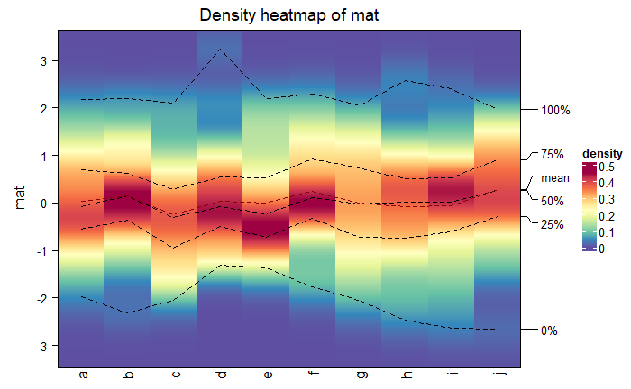
绘制密度分布图

densityHeatmap(mat)

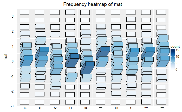
绘制密度直方图

frequencyHeatmap(mat)

为了进一步让热图呈现出3D，使用use_3d = TRUE进行修改参数

frequencyHeatmap(mat, use_3d = TRUE)

6.3 如何实现3D热图呢？

在ComplexHeatmap文档中，也说给出的如何实现3D热图的实例及原理。我们作为初学者也可以简单的学习一下，我们这里说的是简单的学习不需要我们深入的学习。为什么呢？我们并不是作为开发者的角度，我们只是作为使用者。

简单的3D图形

bar3D(x = 0.5, y = 0.5, w = 0.2, h = 0.2, l = unit(1, "cm"), theta = 60)

x: x coordinate of the center point in the bottom face. Value should be a unit object. If it is numeric, the default unit is npc.
y: y coordinate of the center point in the bottom face.
w: Width of the bar (in the x direction). See the following figure.
h: Height of the bar (in the y direction). See the following figure.
l: Length of the bar (in the z direction). See the following figure.
theta: Angle for the projection. See the following figure. Note theta can only take value between 0 and 90.

简单的总结：就是设置长,宽,高以及角度的方向。

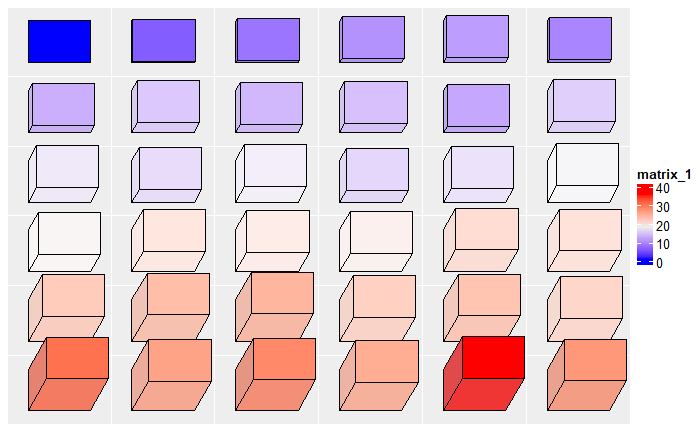
填充颜色

bar3D(x = seq(0.2, 0.8, length = 4), y = 0.5, w = unit(5, "mm"), h = unit(5, "mm"), 
    l = unit(1, "cm"), fill = c("red", "green", "blue", "purple"))

6.4 Heatmap3D()函数使用

实例：

set.seed(7)
mat = matrix(runif(100), 10)
rownames(mat) = LETTERS[1:10]
colnames(mat) = letters[1:10]
Heatmap3D(mat, name = "mat", column_title = "This is a 3D heatmap")

mat = readRDS(system.file("extdata", "measles.rds", package = "ComplexHeatmap"))
year_text = as.numeric(colnames(mat))
year_text[year_text %% 10 != 0] = ""
ha_column = HeatmapAnnotation(
    year = anno_text(year_text, rot = 0, location = unit(1, "npc"), just = "top")
)
## 修改颜色
col_fun = circlize::colorRamp2(c(0, 800, 1000, 127000), c("white", "cornflowerblue", "yellow", "red"))
ht_opt$TITLE_PADDING = unit(c(15, 2), "mm")

Heatmap3D(mat, name = "cases", 
          col = col_fun,
    cluster_columns = FALSE, 
    show_row_dend = FALSE, 
    show_column_names = FALSE,
    row_names_side = "left", row_names_gp = gpar(fontsize = 8),
    column_title = 'Measles cases in US states 1930-2001\nVaccine introduced 1961',
    bottom_annotation = ha_column,
    heatmap_legend_param = list(at = c(0, 5e4, 1e5, 1.5e5), 
        labels = c("0", "50k", "100k", "150k")),
    # new arguments for Heatmap3D()
    bar_rel_width = 1, bar_rel_height = 1, bar_max_length = unit(2, "cm")
)

6.5 补充

对于3D热图的绘制，Jokergoo也在评论区进行一个问题的补充说明

library(ComplexHeatmap)
library(circlize)

m = matrix(1:36, nrow = 6, byrow = TRUE)
m = t(apply(m, 1, sample))
      
      
Heatmap3D(m, cluster_rows = FALSE, cluster_columns = FALSE)

m2 = t(scale(t(m)))

col_fun = colorRamp2(c(-1.5, 0, 1.5), c("blue", "white", "red"))

Heatmap(m2, col = col_fun, rect_gp = gpar(type = "none"),
    layer_fun = function(j, i, x, y, w, h, f) {
        v = pindex(m, i, j)
        od = rank(order(-as.numeric(y), -as.numeric(x)))
        grid.rect(x[od], y[od], w[od], h[od], gp = gpar(col = "white",
            fill = "#EEEEEE"))
        bar3D(x[od], y[od], w[od] * 0.6, h[od] * 0.6, v[od]/max(m) * unit(1, "cm"),
            fill = f[od])
    }, cluster_rows = FALSE, cluster_columns = FALSE)

往期文章：

1. 复现SCI文章系列专栏

2. 《生信知识库订阅须知》,同步更新，易于搜索与管理。

3. 最全WGCNA教程（替换数据即可出全部结果与图形）

4. 精美图形绘制教程

精美图形绘制教程

5. 转录组分析教程

转录组上游分析教程[零基础]

一个转录组上游分析流程 | Hisat2-Stringtie

小杜的生信筆記 ，主要发表或收录生物信息学的教程，以及基于R的分析和可视化（包括数据分析，图形绘制等）；分享感兴趣的文献和学习资料!!

小杜的生信筆記

关注

20
点赞
踩
22

收藏

觉得还不错? 一键收藏
打赏
0
评论
ComplexHeatmap热图专栏 | 6. 3D热图绘制教程

基于《热图绘制教程》专栏，本教程已更新了5个章节，不知道大家是否有所收获。对于小杜个人来说，真的需要不断的复习和练习才可以记住，但是在自己使用的时候也需要重复的看自己的学习笔记。，主要发表或收录生物信息学的教程，以及基于R的分析和可视化（包括数据分析，图形绘制等）；文档中，也说给出的如何实现3D热图的实例及原理。《热图绘制教程》专栏我们通说更新发哦《生信知识库》中，你可以到知识库中查看和学习。不需要我们深入的学习。我们并不是作为开发者的角度，我们只是作为使用者。6 3D热图的绘制教程。对于3D热图的绘制，
复制链接

扫一扫