


 本教程介绍了WGCNA分析的流程,包括样本数据过滤、去除离群值、软阈值选择、模块可视化和模块与表型数据的相关性分析。通过R语言提供的WGCNA包,展示了如何进行基因表达数据的处理和模块构建,并提供了代码示例。教程还提到了如何利用Cytoscape展示hub基因的网络图,并强调了不同参数对结果的影响。
–
关于WGNCA的教程,本次的共有三期教程,我们同时做了三个分析的比较,差异性相对还是比较大的,详情可看WGCNA分析 | 你的数据结果真的是准确的吗??,这里面我们只是做了输出图形的比较差异,具体基因的差异尚未做。如果,有同学感兴趣的话,可以自己做一下。
在前面的教程,我们分享了WGCNA分析 | 全流程分析代码 | 代码一,这个教程的代码就是无脑运行即可,只需要你更改你的输入文件名称即可,后续的参数自己进行调整,基本就可以做结束整个WGCNA的分析,以及获得你想要的结果文件。
本次是WGCNA分析 | 全流程分析代码 | 代码二的教程,本次使用的代码输出的结果与上一次的结果文件类型是一致,但是由于各个方面的参数调整,让结果图形也有不同的改变。
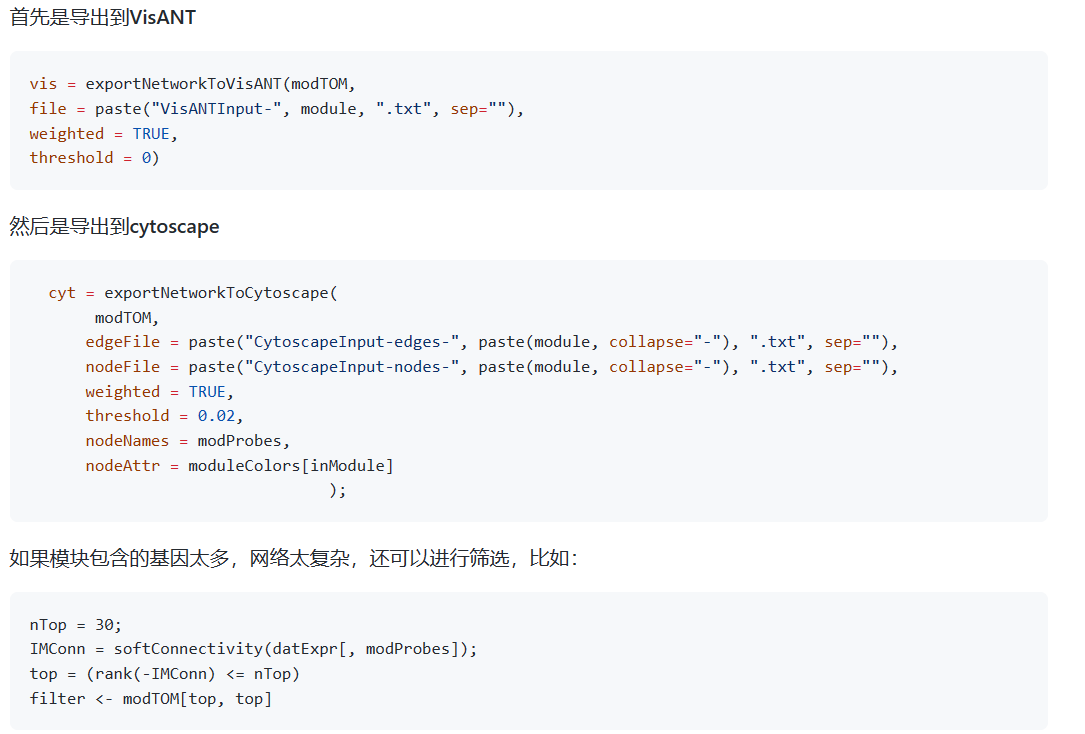
此外,本次教程输出结果多增加了各hub基因之间的Link连接信息。这部分信息,可以直接输入Cytoscape软件中,获得hub的网络图。
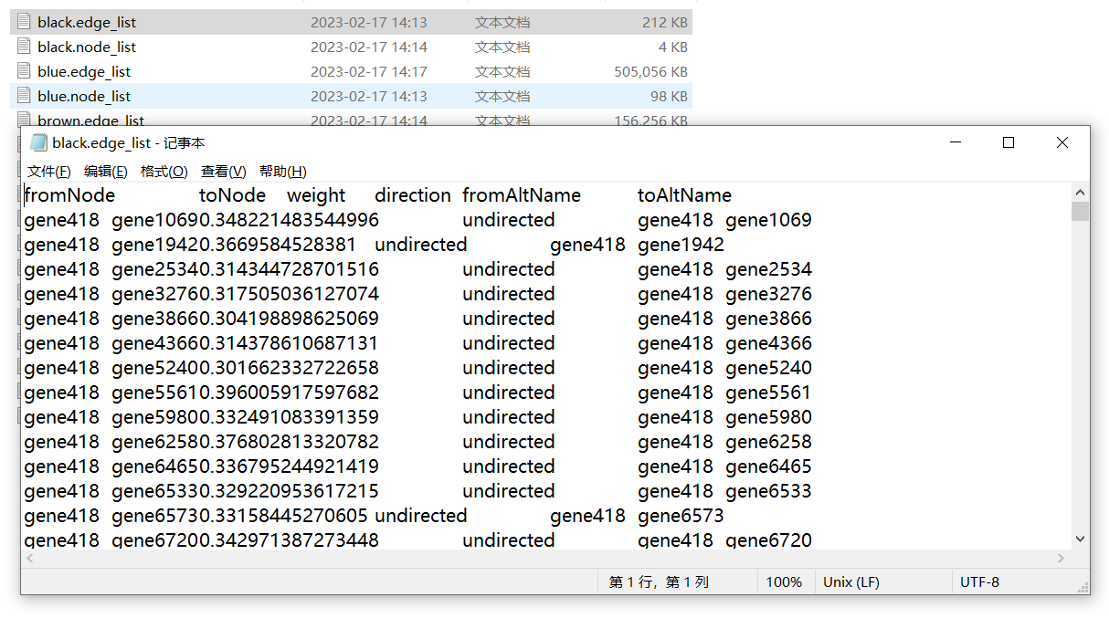
对于这部分数据的输出,参考GitHub中大佬的方法也可以,原理都是一样的。只是本次教程中的代码是批量运行获得全部模块基因的link信息。

1. 教程代码
分析所需包的安装
#install.packages("WGCNA")
#BiocManager::install('WGCNA')

library(WGCNA)
options(stringsAsFactors = FALSE)
## 打开多线程
enableWGCNAThreads()
1.1 样本数据的过滤
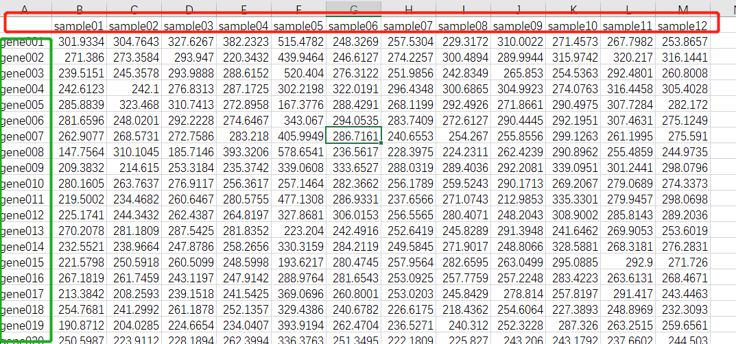
导入数据及处理
exr1_symbol_no_dup <- read.csv("ExpData_WGCNA.csv",row.names = 1)
dim(exr1_symbol_no_dup)
head(exr1_symbol_no_dup)
colnames(exr1_symbol_no_dup)
#转置
mydata <- exr1_symbol_no_dup
datExpr2 = data.frame(t(exr1_symbol_no_dup))
colnames(datExpr2) <- rownames(mydata)
rownames(datExpr2) <- colnames(mydata)
head(datExpr2)
dim(datExpr2)

注:如果你的数据开始就是这里类型的数据格式,即无需进行的此步骤。
基因过滤
datExpr1<-datExpr2
gsg = goodSamplesGenes(datExpr1, verbose = 3);
gsg$allOK
if (!gsg$allOK){
  # Optionally, print the gene and sample names that were removed:
  if (sum(!gsg$goodGenes)>0)
    printFlush(paste("Removing genes:", paste(names(datExpr1)[!gsg$goodGenes], collapse = ", ")));
  if (sum(!gsg$goodSamples)>0)
    printFlush(paste("Removing samples:", paste(rownames(datExpr1)[!gsg$goodSamples], collapse = ", ")));
  # Remove the offending genes and samples from the data:
  datExpr1 = datExpr1[gsg$goodSamples, gsg$goodGenes]
}
绘制样本聚类图
sampleTree = hclust(dist(datExpr1), method = "average")
pdf("1_sample clutering.pdf", width = 6, height = 4)
par(cex = 0.7);
par(mar = c(0,4,2,0))
plot(sampleTree, main = "Sample clustering to detect outliers", sub="", xlab="", cex.lab = 1.5,
     cex.axis = 1.5, cex.main = 2)
dev.off()
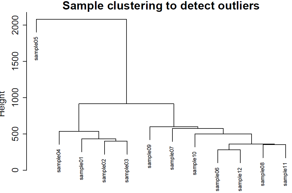
1.2 去除离群体
在样本群体中,有一个样本的是较为离散的,需要去除,我们使用过滤掉Height 高于1500的群体。(注意:abline的参数依据你的数据进行设置。)
pdf("2_sample clutering_delete_outliers.pdf", width = 8, height = 6)
plot(sampleTree, main = "Sample clustering to detect outliers", sub="", xlab="", cex.lab = 1.5,
     cex.axis = 1.5, cex.main = 2) +
  abline(h = 1500, col = "red")  ## abline的参数依据你的数据进行设置
dev.off()

clust = cutreeStatic(sampleTree, cutHeight = 1500, ##cutHeight依据自己的数据设置
                     minSize = 10)
keepSamples = (clust==1)
datExpr = datExpr1[keepSamples, ]
nGenes = ncol(datExpr)
nSamples = nrow(datExpr)
dim(datExpr)
head(datExpr)
####
datExpr0 <- datExpr
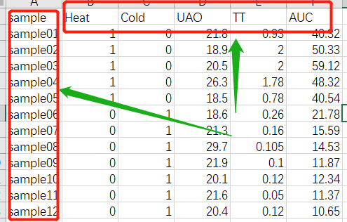
1.3 输入表型数据
############### 载入性状数据## input trait data###############
traitData = read.csv("TraitData.csv",row.names=1)
head(traitData)
allTraits = traitData
dim(allTraits)
names(allTraits)
# 形成一个类似于表达数据的数据框架
fpkmSamples = rownames(datExpr0)
traitSamples =rownames(allTraits)
traitRows = match(fpkmSamples, traitSamples)
datTraits = allTraits[traitRows,]
rownames(datTraits)
collectGarbage()
形成一个类似于表达数据的数据框架
进行二次样本聚类
sampleTree2 = hclust(dist(datExpr), method = "average")
#
traitColors = numbers2colors(datTraits, signed = FALSE)
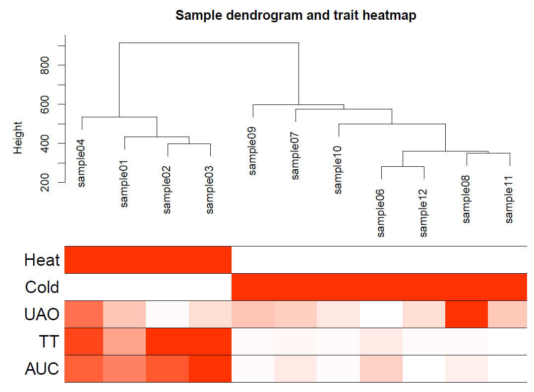
绘制聚类图
pdf(file="3_Sample_dendrogram_and_trait_heatmap.pdf",width=8,height=6)
plotDendroAndColors(sampleTree2, traitColors,
                    groupLabels = names(datTraits),
                    main = "Sample dendrogram and trait heatmap",cex.colorLabels = 1.5, cex.dendroLabels = 1, cex.rowText = 2)
dev.off()
2. 筛选软阈值
soft power一直是WGCNA分析中比较重要的参数,在前面的教程中也讲述过soft power值可以选用软件默认为最好的soft power值,也可以我们自己进行筛选。
enableWGCNAThreads()
# Choose a set of soft-thresholding powers
#powers = c(1:30)
powers = c(c(1:10), seq(from = 12, to=30, by=2))
# Call the network topology analysis function
sft = pickSoftThreshold(datExpr, powerVector = powers, verbose = 5)
绘图soft power plot
pdf(file="4_软阈值选择.pdf",width=12,height= 8)
par(mfrow = c(1,2))
cex1 = 0.85
plot(sft$fitIndices[,1], -sign(sft$fitIndices[,3])*sft$fitIndices[,2],
     xlab="Soft Threshold (power)",ylab="Scale Free Topology Model Fit,signed R^2",type="n",
     main = paste("Scale independence"));
text(sft$fitIndices[,1], -sign(sft$fitIndices[,3])*sft$fitIndices[,2],
     labels=powers,cex=cex1,col="red");
# this line corresponds to using an R^2 cut-off of h
abline(h=0.85,col="red")
# Mean connectivity as a function of the soft-thresholding power
plot(sft$fitIndices[,1], sft$fitIndices[,5],
     xlab="Soft Threshold (power)",ylab="Mean Connectivity", type="n",
     main = paste("Mean connectivity"))
text(sft$fitIndices[,1], sft$fitIndices[,5], labels=powers, cex=cex1,col="red")
dev.off()
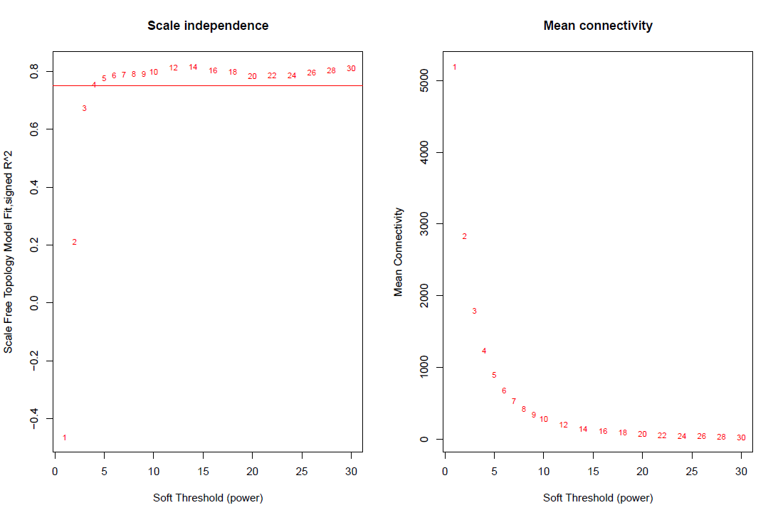
选择最优的soft power值
#softPower =sft$powerEstimate
sft$powerEstimate
softPower = 14
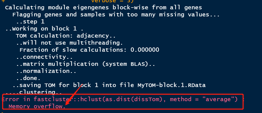
3. 模块可视化
此步耗费较长的时间,敬请等待即可。如果数量较大,建议使用服务器进行分析,不提倡使用的本地进行分析;如果,数据量量较少,本地也可以分析。
net = blockwiseModules(datExpr, power = 6,#手动改power
                       #signed, unsigned
                       TOMType = "signed", minModuleSize = 30,#20, 25
                       reassignThreshold = 0, mergeCutHeight = 0.25, #mergecutheight 0.25
                       numericLabels = TRUE, pamRespectsDendro = FALSE,
                       saveTOMs = TRUE,maxBlockSize = 20000,
                       saveTOMFileBase = "MyTOM",
                       verbose = 3)
table(net$colors)
如果你的数据量较大,或是你的电脑配置内存较小时,可能会出现以下这种情况哦!
绘制模块聚类图
mergedColors = labels2colors(net$colors)
table(mergedColors)
pdf(file="5_Dynamic Tree Cut.pdf",width=8,height=6)
plotDendroAndColors(net$dendrograms[[1]], mergedColors[net$blockGenes[[1]]],
                    "Module colors",
                    dendroLabels = FALSE, hang = 0.03,
                    addGuide = TRUE, guideHang = 0.05)
dev.off()

3.1 模块的合并
如果你这里的模块较多,可以使用前面的教程进行模块的合并即可。具体设置,请看WGCNA分析 | 全流程分析代码 | 代码一
# 合并
merge = mergeCloseModules(datExpr0, dynamicColors, cutHeight = MEDissThres, verbose = 3)
# The merged module colors
mergedColors = merge$colors
# Eigengenes of the new merged modules:
mergedMEs = merge$newMEs
table(mergedColors)

#sizeGrWindow(12, 9)
pdf(file="7_merged dynamic.pdf", width = 9, height = 6)
plotDendroAndColors(geneTree, cbind(dynamicColors, mergedColors),
                    c("Dynamic Tree Cut", "Merged dynamic"),
                    dendroLabels = FALSE, hang = 0.03,
                    addGuide = TRUE, guideHang = 0.05)
dev.off()
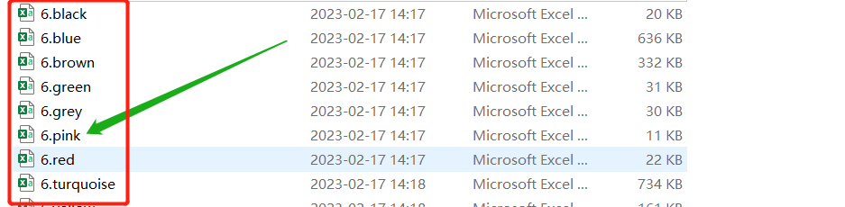
3.2 输出所有的模块基因
moduleLabels = net$colors
moduleColors = labels2colors(net$colors)
MEs = net$MEs
geneTree = net$dendrograms[[1]]
#输出所有modules

color<-unique(moduleColors)
for (i  in 1:length(color)) {
  y=t(assign(paste(color[i],"expr",sep = "."),datExpr[moduleColors==color[i]]))
  write.csv(y,paste('6',color[i],"csv",sep = "."),quote = F)
}

save.image(file = "module_splitted.RData")
load("module_splitted.RData")
4. 模块和表型数据的相关性热图
## 表型
#samples <- read.csv("TraitData.csv",row.names = 1,header = T)
samples <- traitData
samples <- samples[, -(6:6)]
print(samples)
### ----------------------------------------------------------------------------
##        (最重要的) 模块和性状的关系
moduleLabelsAutomatic <-  net$colors
moduleColorsAutomatic <-  labels2colors(moduleLabelsAutomatic)
moduleColorsWW <-  moduleColorsAutomatic
MEs0 <-  moduleEigengenes(datExpr, moduleColorsWW)$eigengenes
## 赋值,后续可能用得到
moduleColors = moduleColorsWW
####
MEsWW <-  orderMEs(MEs0)
modTraitCor <-  cor(MEsWW, samples, use = "p")
colnames(MEsWW)
###赋值
modlues = MEsWW
#write.csv(modlues,file = "./modules_expr.csv")
modTraitP <-  corPvalueStudent(modTraitCor, nSamples)
textMatrix <- paste(signif(modTraitCor, 2), "\n(", signif(modTraitP, 1), ")", sep = "")
dim(textMatrix) <-  dim(modTraitCor)
绘Module-trait图
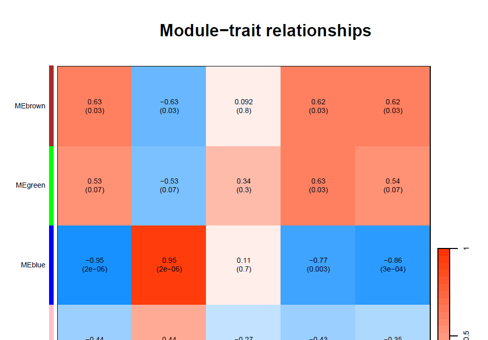
详细内容请查看: WGCNA分析 | 全流程分析代码 | 代码二
小杜的生信筆記 ,主要发表或收录生物信息学的教程,以及基于R的分析和可视化(包括数据分析,图形绘制等);分享感兴趣的文献和学习资料!!


 7129
7129

 被折叠的 条评论
为什么被折叠?
被折叠的 条评论
为什么被折叠?
 到【灌水乐园】发言


