时间序列（四）ARIMA模型与差分

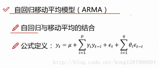
ARIMA模型

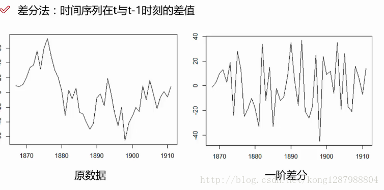
平稳性：
平稳性就是要求经由样本时间序列所得到的拟合曲线
在未来的一段期间内仍能顺着现有的形态“惯性”地延续下去

平稳性要求序列的均值和方差不发生明显变化

严平稳与弱平稳：
严平稳：严平稳表示的分布不随时间的改变而改变。
弱平稳：期望与相关系数（依赖性）不变
未来某时刻的t的值Xt就要依赖于它过去的信息，所以需要依赖性

import pandas as pd
import numpy as np
# Display and Plotting
import matplotlib.pylab as plt
import seaborn as sns

#Read the data
#美国消费者信心指数
Sentiment = 'data/sentiment.csv'
Sentiment = pd.read_csv(Sentiment, index_col=0, parse_dates=[0])
print(Sentiment.head())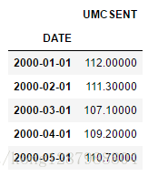

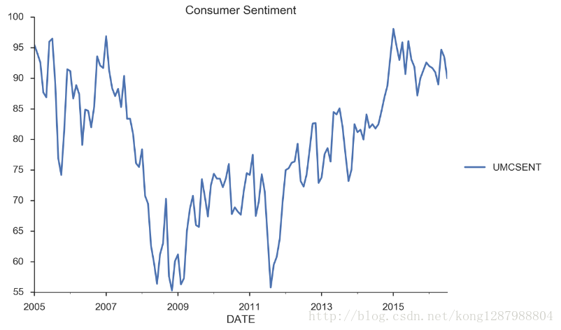
截取其中2005-2016年

# Select the series from 2005 - 2016
sentiment_short = Sentiment.loc['2005':'2016']

sentiment_short.plot(figsize=(12,8))
plt.legend(bbox_to_anchor=(1.25, 0.5))
plt.title("Consumer Sentiment")
sns.despine()
plot.show()

画出来

画出一阶差分与二阶差分的图

sentiment_short['diff_1'] = sentiment_short['UMCSENT'].diff(1)

sentiment_short['diff_2'] = sentiment_short['diff_1'].diff(1)

sentiment_short.plot(subplots=True, figsize=(18, 12))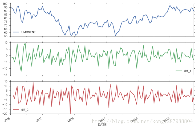

ARIMA模型原理

自回归模型AR
描述当前值与历史值之间的关系，用变量自身的历史时间数据对自身进行预测
自回归模型必须满足平稳性的要求
p阶自回归过程的公式定义：

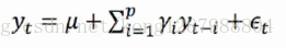
yt是当前值 u是常数项 P是阶数 ri是自相关系数 et是误差
（P当前值距p天前的值的关系）

自回归模型的限制
1、自回归模型是用自身的数据进行预测
2、必须具有平稳性
3、必须具有相关性，如果自相关系数（φi）小于0.5，则不宜采用
4、自回归只适用于预测与自身前期相关的现象

移动平均模型MA
移动平均模型关注的是自回归模型中的误差项的累加
q阶自回归过程的公式定义：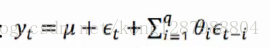
移动平均法能有效地消除预测中的随机波动

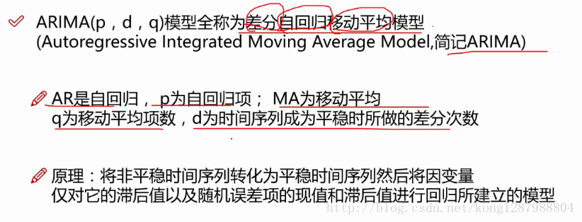
I是差分模型

需要确定P和Q，
d是做几阶差分,一般1阶就可以了

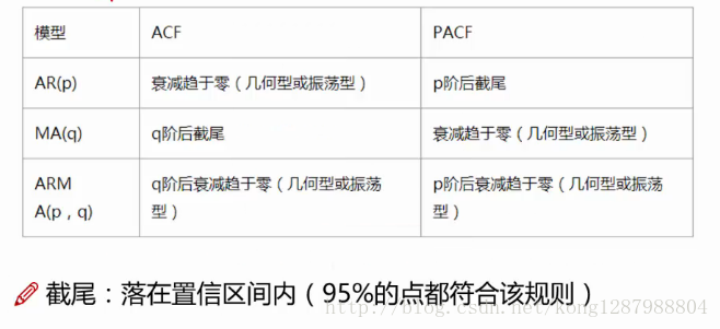
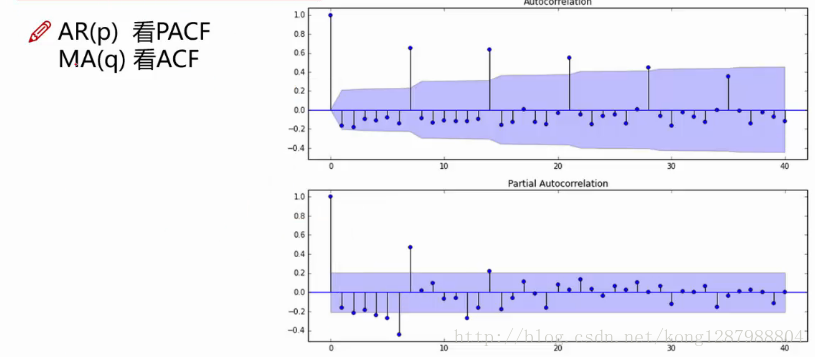
选择P与Q的方法：
自相关函数ACF（autocorrelation function）
有序的随机变量序列与其自身相比较自相关函数反映了同一序列在不同时序的取值的相关性
公式：

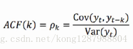
变量与自身的变化，yt和yt-1到yt和yt-k的相关系数
k阶滞后点
Pk的取值范围【-1，1】

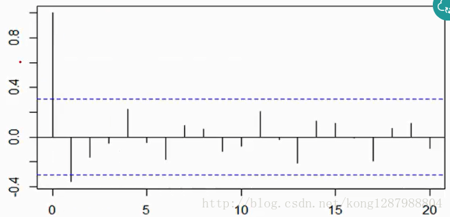
虚线表示95%，置信区间

偏自相关函数（PACF）（partial autocorrelation function）
1、对于一个平稳AR（p）模型，求出滞后k自相关系数p（k）时
实际上得到的并不是x（t）与x（t-k）之间单纯的相关关系
2、x（t）同时还会受到中间k-1个随机变量x（t-1）、x（t-2）……、x（t-k+1）的影响，而这k-1个随机变量又都和x（t-k）具有相关关系，所以自相关系数p（k）里实际掺杂了其他变量对x（t）与x（t-k）的影响
3、剔除了中间k-1个随机变量x（t-1）、x（t-2）、……、x（t-k+1）的干扰之后
x（t-k）对x（t）影响的相关程度
4、ACF还包含了其他变量的影响
而偏自相关系数PACF是严格这两个变量之间的相关性

需要用到模块statsmodels

# TSA from Statsmodels
import statsmodels.api as sm
import statsmodels.formula.api as smf
import statsmodels.tsa.api as smt

分别画出ACF和PACF图像

fig = plt.figure(figsize=(12,8))

ax1 = fig.add_subplot(211)
fig = sm.graphics.tsa.plot_acf(sentiment_short, lags=20,ax=ax1)
ax1.xaxis.set_ticks_position('bottom')
fig.tight_layout();

ax2 = fig.add_subplot(212)
fig = sm.graphics.tsa.plot_pacf(sentiment_short, lags=20, ax=ax2)
ax2.xaxis.set_ticks_position('bottom')
fig.tight_layout();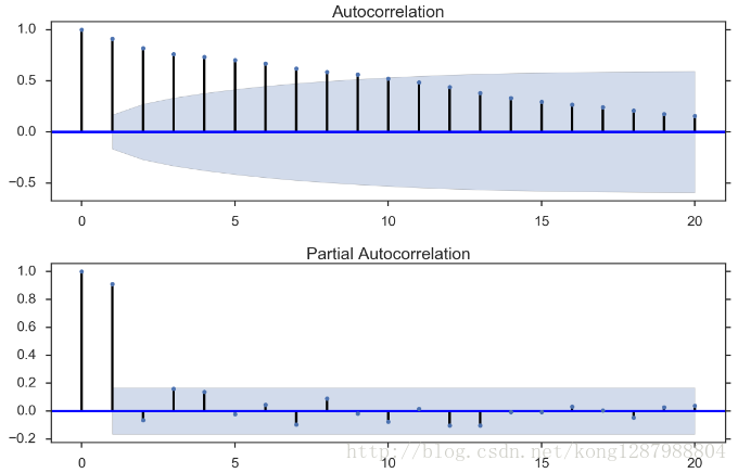

接下来确定ARIMA模型的p、d、q三个参数
ARIMA(p,d,q)
确认方法：

例子：

四个图的整合函数，可以改参数直接调用

# 更直观一些

def tsplot(y, lags=None, title='', figsize=(14, 8)):

    fig = plt.figure(figsize=figsize)
    layout = (2, 2)
    ts_ax   = plt.subplot2grid(layout, (0, 0))
    hist_ax = plt.subplot2grid(layout, (0, 1))
    acf_ax  = plt.subplot2grid(layout, (1, 0))
    pacf_ax = plt.subplot2grid(layout, (1, 1))

    y.plot(ax=ts_ax)
    ts_ax.set_title(title)
    y.plot(ax=hist_ax, kind='hist', bins=25)
    hist_ax.set_title('Histogram')
    smt.graphics.plot_acf(y, lags=lags, ax=acf_ax)
    smt.graphics.plot_pacf(y, lags=lags, ax=pacf_ax)
    [ax.set_xlim(0) for ax in [acf_ax, pacf_ax]]
    sns.despine()
    plt.tight_layout()
    return ts_ax, acf_ax, pacf_ax

使用：

tsplot(sentiment_short, title='Consumer Sentiment', lags=36);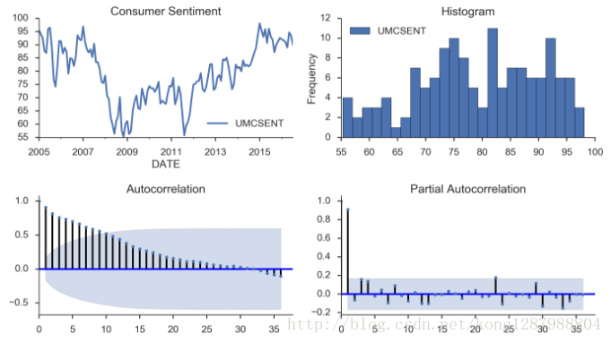

另一种判别：

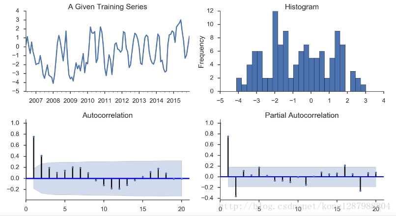
从图中可以看出p=2，d=0，q=0 较为合适
于是训练模型

#Model Estimation

# Fit the model
arima200 = sm.tsa.SARIMAX(ts_train, order=(2,0,0))
model_results=arima200.fit()

通过导入import itertools来遍历

import itertools

p_min = 0
d_min = 0
q_min = 0
p_max = 4
d_max = 0
q_max = 4

# Initialize a DataFrame to store the results
results_bic = pd.DataFrame(index=['AR{}'.format(i) for i in range(p_min,p_max+1)],
                           columns=['MA{}'.format(i) for i in range(q_min,q_max+1)])

for p,d,q in itertools.product(range(p_min,p_max+1),
                               range(d_min,d_max+1),
                               range(q_min,q_max+1)):
    if p==0 and d==0 and q==0:
        results_bic.loc['AR{}'.format(p), 'MA{}'.format(q)] = np.nan
        continue

    try:
        model = sm.tsa.SARIMAX(ts_train, order=(p, d, q),
                               #enforce_stationarity=False,
                               #enforce_invertibility=False,
                              )
        results = model.fit()
        results_bic.loc['AR{}'.format(p), 'MA{}'.format(q)] = results.bic
    except:
        continue
results_bic = results_bic[results_bic.columns].astype(float)

画出热度图

fig, ax = plt.subplots(figsize=(10, 8))
ax = sns.heatmap(results_bic,
                 mask=results_bic.isnull(),
                 ax=ax,
                 annot=True,
                 fmt='.2f',
                 );
ax.set_title('BIC');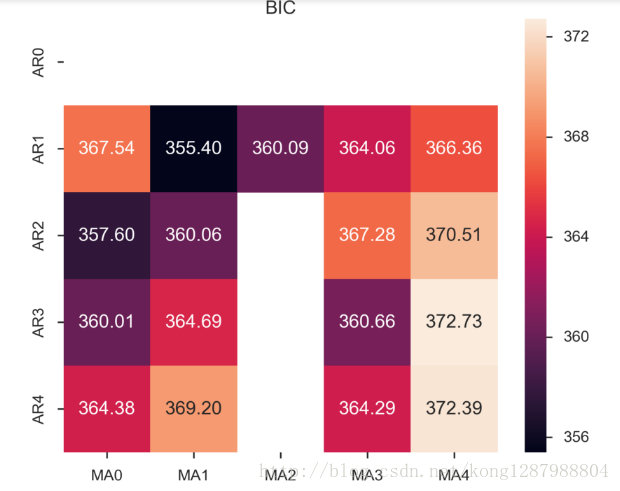

输出AIC、BIC评价指标

# Alternative model selection method, limited to only searching AR and MA parameters

train_results = sm.tsa.arma_order_select_ic(ts_train, ic=['aic', 'bic'], trend='nc', max_ar=4, max_ma=4)

print('AIC', train_results.aic_min_order)
print('BIC', train_results.bic_min_order)

AIC (4, 2)
BIC (1, 1)
结果不一致需要我们重新审判

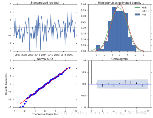
#残差分析 正态分布 QQ图线性
model_results.plot_diagnostics(figsize=(16, 12));

分析其他指标