


霍夫变换
在图像x-y坐标中,经过点(x_i, y_i)的直线表示为y_i=k∗ x_i+b (1),其中k为斜率,b为截距
如果将x_i 、y_i 看成常数,把k和b看成变量,式子(1)可以表示为b = - k∗ x_i + y_i(2)
这样就把点(x_i, y_i)在图像坐标空间x-y中的表示转变成为了参数空间a-b中的表示,这个过程被称为Hough变换
霍夫直线变换
原理解析

一个斜率和一个截距确定一条直线,但是斜率有可能不存在,因此可以转化为用 Θ \Theta Θ 和 r r r 表示 ,将(x,y)做hough变换可以得到参数空间下的方程。
那么,( Θ \Theta Θ , r r r)就是参数空间的一个点,(x,y)则确定了过该点的直线。经过点( Θ \Theta Θ , r r r)的直线越多,证明确定这些直线的点 ( x i , y i ) (x_i, y_i) (xi,yi)共线的可能性越大,因此需要统计每个( Θ \Theta Θ , r r r)上有直线经过的次数。这个统计器就对应了复现代码中的accumulator。
得到统计器后,则需要确定一个阈值,统计器上对应位置的值若超过该阈值,则认为此参数( Θ i {\Theta}_i Θi , r i r_i ri)可以确定直线坐标空间的一条直线
根据确定的参数( Θ i {\Theta}_i Θi , r i r_i ri),在原图上做出直线即可。
实验
原图:

canny边缘检测:

不加极大值抑制:

加了非极大值抑制:

代码解读
python代码库实现
     # hough直线变换python库实现
    lines = cv2.HoughLines(imgEdge, 1, np.pi / 180, 160) # 1和np.pi / 180分别是投票矩阵的最小单位
    lines1 = lines[:, 0, :]  # 提取为二维
    for rho, theta in lines1[:]: # 取出lines每一行的两个数
        a = np.cos(theta)
        b = np.sin(theta)
        x0 = a * rho # (x0,y0)是参数方程r = x * cos(theta) + y * sin(theta)恒过的点)
        y0 = b * rho
        # 利用theta和rho、已知的一个点(x0,y0)来确定直线上的另外两个点,1000是随便取的值
        x1 = int(x0 + 1000 * (-b))
        y1 = int(y0 + 1000 * (a))
        x2 = int(x0 - 1000 * (-b))
        y2 = int(y0 - 1000 * (a))
        cv2.line(img, (x1, y1), (x2, y2), (255, 0, 0), 1) # 1是调节直线的宽度
	plt.imshow(img, cmap="gray")
    plt.axis("off")  # 关闭坐标
    plt.show()
注意 ( x 0 , y 0 ) (x_0 , y_0) (x0,y0)是利用极坐标求出来的点(高中知识)
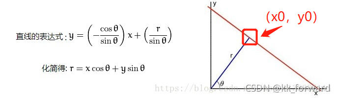
知道 ( x 0 , y 0 ) (x_0 , y_0) (x0,y0) 后,就可以根据下图的原理,求出该直线任意的两个点 ( x 1 , y 1 (x_1,y_1 (x1,y1)、 ( x 2 , y 2 (x_2,y_2 (x2,y2):

代码复现:
def lineHough(imgEdge, thetaDim = None,threshold = None):
    """
    :param imgEdge: 输入的经过边缘检测后的图像
    :param ThetaDim: Theta轴的刻度数量(将(0,pi)划分成多少份),若为90则分为90份,每份为2
    :param threshold: 投票界定是否为直线的阈值
    :return: 符合阈值的投票箱结果
    """
    imgsize = imgEdge.shape
    if thetaDim == None:
        ThetaDim = 180
    MaxDist = int(np.ceil(np.sqrt(imgsize[0] ** 2 + imgsize[1] ** 2)))

    accumulator = np.zeros((ThetaDim, MaxDist))  # theta的范围是[0,pi). 在这里将[0,pi)进行了线性映射.类似的,也对Dist轴进行了线性映射

    sinTheta = [np.sin(t * np.pi / ThetaDim) for t in range(ThetaDim)]
    cosTheta = [np.cos(t * np.pi / ThetaDim) for t in range(ThetaDim)]

    for i in range(imgsize[0]):
        for j in range(imgsize[1]):
            if not imgEdge[i, j] == 0:
                for k in range(ThetaDim):
                    accumulator[k][int(round((i * cosTheta[k] + j * sinTheta[k])))] += 1

    M = accumulator.max()

    if threshold == None:
        threshold = int(M * 2.3875 / 10)
    result = np.array(np.where(accumulator > threshold))  # 阈值化
    result = result.astype(np.float64)
    result[0] = result[0] * np.pi / ThetaDim
    return result

def drawLine(line, img, color = (255, 0, 0), err = 6):
        """

    :param line: lineHough返回的结果
    :param img: 原图片
    :param color: 画线的颜色
    :param err: 误差大小,可调
    :return: 返回画线后的图片
    """
    Cos = np.cos(line[0])
    Sin = np.sin(line[0])

    # 遍历img中像素的所有位置,再将该位置坐标带入参数方程中(因为该俩参数是可以确定直线的,所以满足该方程则证明该点一定在某条直线上)
    # 这里.any()是需要两个矩阵中有一个数相等就行,是属于判断两个矩阵相等的技巧
    # 这里的误差是做hough变换的时候,做一些数字运算例如四舍五入,取整之类带来的,所以一定是有误差存在的
    for i in range(img.shape[0]):
        for j in range(img.shape[1]):
            e = np.abs(line[1] - i * Cos - j * Sin)
            if (e < err).any():
                img[i, j] = color
    return img
注意这里画图的方式与python库画图的方式不一样,这里是遍历每个点,判断每个点是否符合参数方程,而python库是随机挑选两个点,然后连接这两点画图
霍夫圆变换
原理解析
Hough梯度法
圆检测需要确定三个参数 :(圆心横坐标,圆心中坐标,半径长度),若在三维空间计算,时间很长。可以把霍夫变换分解为两个阶段,减少维度。
第一阶段检测圆心:若同一个圆周上的点,则这些点的梯度方向都应该交于圆心。因此可以对边缘点求梯度,获得梯度方向上的直线,对直线相交点数进行累加,累加数较多的位置点则认为是候选圆心。
第二阶段检测半径:求得圆心的位置后,圆周上的点到圆心的距离相等。因此可以对每个边缘点求一次到候选圆心的距离,同一个距离的点数进行累加,累加数较多的距离则认为是候选半径。
确定圆心
作图是原图像,右图是原图像边缘点的梯度方向直线。亮处为相交次数最多的点,以此确定圆心。


实验


图一是原图像,图2是经过canny提取边缘后的图像,图3是边缘点梯度方向的直线,图4hough圆检测结果图
代码解读:
python代码库实现
gray = cv2.cvtColor(img, cv2.COLOR_RGB2GRAY)
cv2.waitKey(0)
# 参数:gray:输入的灰度图像;求解方法;图像像素分辨率与参数空间分辨率的比值;检测到的圆的中心,(x,y)坐标之间的最小距离;param1:用于处理边缘检测的梯度值方法;
# param2:累加器阈值。阈值越小,检测到的圆越多;半径的最小大小(以像素为单位;半径的最大大小(以像素为单位)
circles = cv2.HoughCircles(gray, cv2.HOUGH_GRADIENT, 1, 100, param1 = 150,
                           param2=30, minRadius=350, maxRadius=600)
circle = circles[0, :, :] # 提取为二维
circle = np.uint16(np.around(circle))
for i in circle[:]:
    cv2.circle(img, (i[0], i[1]), i[2], (0,0,255),5)
    cv2.circle(img, (i[0], i[1]), 2, (0, 0, 255), 10) # 半径取两个像素点,相当于调整圆心的厚度,最后一个参数是thickness
    plt.imshow(img)
    plt.axis('off')
    plt.show()
缺点:函数中含有很多参数,最后圆检测的好坏跟参数相关性太大,往往每张图片需要调整的参数都相差较远
代码复现
def AHTforCircles(edge,center_threhold_factor = None,score_threhold = None,min_center_dist = None,minRad = None,maxRad = None,center_axis_scale = None,radius_scale = None,halfWindow = None,max_circle_num = None):
    if center_threhold_factor == None:
        center_threhold_factor = 10.0
    if score_threhold == None:
        score_threhold = 15.0
    if min_center_dist == None:
        min_center_dist = 80.0
    if minRad == None:
        minRad = 0.0
    if maxRad == None:
        maxRad = 1e7*1.0
    if center_axis_scale == None:
        center_axis_scale = 1.0
    if radius_scale == None:
        radius_scale = 1.0
    if halfWindow == None:
        halfWindow = 2
    if max_circle_num == None:
        max_circle_num = 6
    min_center_dist_square = min_center_dist**2


    sobel_kernel_y = np.array([[-1.0, -2.0, -1.0], [0.0, 0.0, 0.0], [1.0, 2.0, 1.0]])
    sobel_kernel_x = np.array([[-1.0, 0.0, 1.0], [-2.0, 0.0, 2.0], [-1.0, 0.0, 1.0]])
    # 分别求得在x和y方向上的梯度
    edge_x = convolve(sobel_kernel_x, edge, [1,1,1,1], [1,1])
    edge_y = convolve(sobel_kernel_y, edge, [1,1,1,1], [1,1])


    center_accumulator = np.zeros((int(np.ceil(center_axis_scale*edge.shape[0])),int(np.ceil(center_axis_scale*edge.shape[1]))))
    k = np.array([[r for c in range(center_accumulator.shape[1])] for r in range(center_accumulator.shape[0])])
    l = np.array([[c for c in range(center_accumulator.shape[1])] for r in range(center_accumulator.shape[0])])
    minRad_square = minRad**2
    maxRad_square = maxRad**2
    points = [[],[]] # 存储为edge且点梯度不为0的像素位置下标
    # ((1,1),(1,1)):前面的(1,1)是行填充,第一个1是edge_x的上面填,第二个1是在edge_x的下面填,后面的(1,1)同理
    edge_x_pad = np.pad(edge_x,((1,1),(1,1)),'constant')
    edge_y_pad = np.pad(edge_y,((1,1),(1,1)),'constant')
    Gaussian_filter_3 = 1.0 / 16 * np.array([(1.0, 2.0, 1.0), (2.0, 4.0, 2.0), (1.0, 2.0, 1.0)])
    # 根据梯度方向投票
    for i in range(edge.shape[0]):
        for j in range(edge.shape[1]):
            if not edge[i,j] == 0:
                dx_neibor = edge_x_pad[i:i+3,j:j+3]
                dy_neibor = edge_y_pad[i:i+3,j:j+3]
                dx = (dx_neibor*Gaussian_filter_3).sum()
                dy = (dy_neibor*Gaussian_filter_3).sum()
                if not (dx == 0 and dy == 0): # dx和dy都为0,肯定不是圆周上的点,可以排除
                    t1 = (k/center_axis_scale-i)
                    t2 = (l/center_axis_scale-j)
                    t3 = t1**2 + t2**2
                    # 这里为什么这样求? 这里求出来的t3是所有边缘点的梯度,是512*512,temp是[512,512]的bool矩阵,
                    # center_accumulator[temp] += 1 直接对整个矩阵进行加减了
                    temp = (t3 > minRad_square)&(t3 < maxRad_square)&(np.abs(dx*t1-dy*t2) < 1e-4) #
                    center_accumulator[temp] += 1
                    points[0].append(i)
                    points[1].append(j)

    M = center_accumulator.mean()
    # for i in range(center_accumulator.shape[0]):
    #     for j in range(center_accumulator.shape[1]):
    #         neibor = \
    #             center_accumulator[max(0, i - halfWindow + 1):min(i + halfWindow, center_accumulator.shape[0]),
    #             max(0, j - halfWindow + 1):min(j + halfWindow, center_accumulator.shape[1])]
    #         if not (center_accumulator[i,j] >= neibor).all():
    #             center_accumulator[i,j] = 0
    #                                                                     非极大值抑制
    # 圆心在原图上的分布图
    plt.imshow(center_accumulator)
    plt.axis('off')
    cwd = os.getcwd()
    saveFile = Path(cwd,"image/hough")
    plt.savefig(str(Path(saveFile, "circleImg")))
    plt.show()

    center_threshold = M * center_threhold_factor # 利用均值求得阈值
    possible_centers = np.array(np.where(center_accumulator > center_threshold))  # 阈值化


    sort_centers = []
    for i in range(possible_centers.shape[1]):
        sort_centers.append([])
        sort_centers[-1].append(possible_centers[0,i])
        sort_centers[-1].append(possible_centers[1, i])
        sort_centers[-1].append(center_accumulator[sort_centers[-1][0],sort_centers[-1][1]])
    # 最后sort_centers中的每个list中是[像素矩阵x,像素矩阵y,投票数]
    sort_centers.sort(key=lambda x:x[2],reverse=True) # 按照投票数排序,从大到小

    centers = [[],[],[]]
    points = np.array(points)
    for i in range(len(sort_centers)): # 确定完圆心后,确定半径,这里的radius是一个一维向量,因为只需要确定r的大小即可,而center_accumulator需要确定两个值,所以为2维的
        radius_accumulator = np.zeros( # 半径统计矩阵最大值为对角线
            (int(np.ceil(radius_scale * min(maxRad, np.sqrt(edge.shape[0] ** 2 + edge.shape[1] ** 2)) + 1))),dtype=np.float32)
        if not len(centers[0]) < max_circle_num:
            break
        iscenter = True
        for j in range(len(centers[0])):
            d1 = sort_centers[i][0]/center_axis_scale - centers[0][j]
            d2 = sort_centers[i][1]/center_axis_scale - centers[1][j]
            if d1**2 + d2**2 < min_center_dist_square:
                iscenter = False
                break

        if not iscenter:
            continue
        # temp 是points中每个点到候选圆心的距离
        temp = np.sqrt((points[0,:] - sort_centers[i][0] / center_axis_scale) ** 2 + (points[1,:] - sort_centers[i][1] / center_axis_scale) ** 2)
        temp2 = (temp > minRad) & (temp < maxRad) #temp是一个向量
        temp = (np.round(radius_scale * temp)).astype(np.int32)
        for j in range(temp.shape[0]):
            if temp2[j]:
                radius_accumulator[temp[j]] += 1 # 该距离上的点数+1
        for j in range(radius_accumulator.shape[0]):
            if j == 0 or j == 1:
                continue
            if not radius_accumulator[j] == 0: # np.log(j)是e^j,log是以e为底的对数,有点归一化的感觉
                radius_accumulator[j] = radius_accumulator[j]*radius_scale/np.log(j) #radius_accumulator[j]*radius_scale/j
        score_i = radius_accumulator.argmax(axis=-1) #第几个位置的值最大
        if radius_accumulator[score_i] < score_threhold: # 与阈值做比较,若小于阈值,则不判断为圆心
            iscenter = False

        if iscenter:
            centers[0].append(sort_centers[i][0]/center_axis_scale)
            centers[1].append(sort_centers[i][1]/center_axis_scale)
            # 这里应该是半径,但是为什么返回了radius_accumulator最大值的位置?
            # kang:因为radius_accumulator的长度是0-对角线,存储的是每个位置出现的次数,因此score_i就是对应的半径
            centers[2].append(score_i/radius_scale)


    centers = np.array(centers)
    centers = centers.astype(np.float64)

    return centers
解析:这里的求梯度用了sobel算子,求解过程比直接调库慢许多
参考资料:
https://zengdiqing.blog.csdn.net/article/details/86104053
https://www.bilibili.com/video/BV1bb411b7VQ


 8269
8269


 被折叠的 条评论
为什么被折叠?
被折叠的 条评论
为什么被折叠?
 到【灌水乐园】发言


