


Colab/PyTorch - 002 Pre Trained Models for Image Classification
1. 源由
这篇文章中,我们将深入探讨在TorchVision模块中使用的预训练网络的一些实际示例,图像分类的预训练模型。
Torchvision包含流行的数据集、模型架构以及常用的图像转换功能,用于计算机视觉。
基本上,如果对计算机视觉感兴趣并且正在使用PyTorch,Torchvision将会帮助很大!
2. 图像分类的预训练模型
预训练模型是在诸如ImageNet之类的大型基准数据集上训练的神经网络模型。深度学习社区从这些开源模型中受益匪浅。此外,预训练模型是计算机视觉研究迅速进步的主要因素。其他研究人员和实践者可以使用这些最先进的模型,而不是从头开始重新发明一切。
下面是随着时间推移,最先进模型如何改进的大致时间轴,列出了Torchvision包中存在的那些模型。
 在深入讨论如何使用预训练模型进行图像分类之前,先看看有哪些可用的预训练模型。在这里,将讨论AlexNet和ResNet101这两个主要示例。这两个网络都是在ImageNet数据集上进行训练的。
ImageNet数据集由斯坦福大学维护,拥有超过1400万张图像。它被广泛用于各种图像相关的深度学习项目。这些图像属于各种不同的类别或标签。虽然我们可以互换使用这两个术语,但将坚持使用“类别”。像AlexNet和ResNet101这样的预训练模型的目的是接受一张图像作为输入,并预测其所属的类别。
这里的“预训练”一词意味着深度学习架构,比如AlexNet和ResNet101,已经在某个(庞大的)数据集上进行了训练,并携带了相应的权重和偏差。
3. 示例 - AlexNet/ResNet101
架构与权重和偏差之间的区别应该非常清楚,因为正如将要看到的那样,TorchVision既有架构,也有预训练模型。
3.1 模型推断过程
由于我们将专注于如何使用预训练模型来预测输入的类别(标签),让我们也讨论涉及其中的过程。这个过程被称为模型推断。整个过程包括以下主要步骤:
- 读取输入图像
- 对图像执行转换。例如 - 调整大小、中心裁剪、归一化等。
- 前向传播:使用预训练权重来找出输出向量。输出向量中的每个元素描述了模型预测输入图像属于特定类别的置信度。
- 根据获得的分数(第3步中提到的输出向量的元素),显示预测结果。
3.2 使用TorchVision加载预训练网络
现在已经掌握了模型推断的知识,并知道了预训练模型的含义,让我们看看如何借助TorchVision模块来使用它们。
首先,让我们使用下面给出的命令安装TorchVision模块。
$ pip install torchvision
接下来,让我们从torchvision模块中导入models,并查看我们可以使用的不同模型和架构。
from torchvision import models
import torch

dir(models)
['AlexNet',
 'AlexNet_Weights',
 'ConvNeXt',
 'ConvNeXt_Base_Weights',
 'ConvNeXt_Large_Weights',
 'ConvNeXt_Small_Weights',
 'ConvNeXt_Tiny_Weights',
 'DenseNet',
 'DenseNet121_Weights',
 'DenseNet161_Weights',
 'DenseNet169_Weights',
 'DenseNet201_Weights',
 'EfficientNet',
 'EfficientNet_B0_Weights',
 'EfficientNet_B1_Weights',
 'EfficientNet_B2_Weights',
 'EfficientNet_B3_Weights',
 'EfficientNet_B4_Weights',
 'EfficientNet_B5_Weights',
 'EfficientNet_B6_Weights',
 'EfficientNet_B7_Weights',
 'EfficientNet_V2_L_Weights',
 'EfficientNet_V2_M_Weights',
 'EfficientNet_V2_S_Weights',
 'GoogLeNet',
 'GoogLeNetOutputs',
 'GoogLeNet_Weights',
 'Inception3',
 'InceptionOutputs',
 'Inception_V3_Weights',
 'MNASNet',
 'MNASNet0_5_Weights',
 'MNASNet0_75_Weights',
 'MNASNet1_0_Weights',
 'MNASNet1_3_Weights',
 'MaxVit',
 'MaxVit_T_Weights',
 'MobileNetV2',
 'MobileNetV3',
 'MobileNet_V2_Weights',
 'MobileNet_V3_Large_Weights',
 'MobileNet_V3_Small_Weights',
 'RegNet',
 'RegNet_X_16GF_Weights',
 'RegNet_X_1_6GF_Weights',
 'RegNet_X_32GF_Weights',
 'RegNet_X_3_2GF_Weights',
 'RegNet_X_400MF_Weights',
 'RegNet_X_800MF_Weights',
 'RegNet_X_8GF_Weights',
 'RegNet_Y_128GF_Weights',
 'RegNet_Y_16GF_Weights',
 'RegNet_Y_1_6GF_Weights',
 'RegNet_Y_32GF_Weights',
 'RegNet_Y_3_2GF_Weights',
 'RegNet_Y_400MF_Weights',
 'RegNet_Y_800MF_Weights',
 'RegNet_Y_8GF_Weights',
 'ResNeXt101_32X8D_Weights',
 'ResNeXt101_64X4D_Weights',
 'ResNeXt50_32X4D_Weights',
 'ResNet',
 'ResNet101_Weights',
 'ResNet152_Weights',
 'ResNet18_Weights',
 'ResNet34_Weights',
 'ResNet50_Weights',
 'ShuffleNetV2',
 'ShuffleNet_V2_X0_5_Weights',
 'ShuffleNet_V2_X1_0_Weights',
 'ShuffleNet_V2_X1_5_Weights',
 'ShuffleNet_V2_X2_0_Weights',
 'SqueezeNet',
 'SqueezeNet1_0_Weights',
 'SqueezeNet1_1_Weights',
 'SwinTransformer',
 'Swin_B_Weights',
 'Swin_S_Weights',
 'Swin_T_Weights',
 'Swin_V2_B_Weights',
 'Swin_V2_S_Weights',
 'Swin_V2_T_Weights',
 'VGG',
 'VGG11_BN_Weights',
 'VGG11_Weights',
 'VGG13_BN_Weights',
 'VGG13_Weights',
 'VGG16_BN_Weights',
 'VGG16_Weights',
 'VGG19_BN_Weights',
 'VGG19_Weights',
 'ViT_B_16_Weights',
 'ViT_B_32_Weights',
 'ViT_H_14_Weights',
 'ViT_L_16_Weights',
 'ViT_L_32_Weights',
 'VisionTransformer',
 'Weights',
 'WeightsEnum',
 'Wide_ResNet101_2_Weights',
 'Wide_ResNet50_2_Weights',
 '_GoogLeNetOutputs',
 '_InceptionOutputs',
 '__builtins__',
 '__cached__',
 '__doc__',
 '__file__',
 '__loader__',
 '__name__',
 '__package__',
 '__path__',
 '__spec__',
 '_api',
 '_meta',
 '_utils',
 'alexnet',
 'convnext',
 'convnext_base',
 'convnext_large',
 'convnext_small',
 'convnext_tiny',
 'densenet',
 'densenet121',
 'densenet161',
 'densenet169',
 'densenet201',
 'detection',
 'efficientnet',
 'efficientnet_b0',
 'efficientnet_b1',
 'efficientnet_b2',
 'efficientnet_b3',
 'efficientnet_b4',
 'efficientnet_b5',
 'efficientnet_b6',
 'efficientnet_b7',
 'efficientnet_v2_l',
 'efficientnet_v2_m',
 'efficientnet_v2_s',
 'get_model',
 'get_model_builder',
 'get_model_weights',
 'get_weight',
 'googlenet',
 'inception',
 'inception_v3',
 'list_models',
 'maxvit',
 'maxvit_t',
 'mnasnet',
 'mnasnet0_5',
 'mnasnet0_75',
 'mnasnet1_0',
 'mnasnet1_3',
 'mobilenet',
 'mobilenet_v2',
 'mobilenet_v3_large',
 'mobilenet_v3_small',
 'mobilenetv2',
 'mobilenetv3',
 'optical_flow',
 'quantization',
 'regnet',
 'regnet_x_16gf',
 'regnet_x_1_6gf',
 'regnet_x_32gf',
 'regnet_x_3_2gf',
 'regnet_x_400mf',
 'regnet_x_800mf',
 'regnet_x_8gf',
 'regnet_y_128gf',
 'regnet_y_16gf',
 'regnet_y_1_6gf',
 'regnet_y_32gf',
 'regnet_y_3_2gf',
 'regnet_y_400mf',
 'regnet_y_800mf',
 'regnet_y_8gf',
 'resnet',
 'resnet101',
 'resnet152',
 'resnet18',
 'resnet34',
 'resnet50',
 'resnext101_32x8d',
 'resnext101_64x4d',
 'resnext50_32x4d',
 'segmentation',
 'shufflenet_v2_x0_5',
 'shufflenet_v2_x1_0',
 'shufflenet_v2_x1_5',
 'shufflenet_v2_x2_0',
 'shufflenetv2',
 'squeezenet',
 'squeezenet1_0',
 'squeezenet1_1',
 'swin_b',
 'swin_s',
 'swin_t',
 'swin_transformer',
 'swin_v2_b',
 'swin_v2_s',
 'swin_v2_t',
 'vgg',
 'vgg11',
 'vgg11_bn',
 'vgg13',
 'vgg13_bn',
 'vgg16',
 'vgg16_bn',
 'vgg19',
 'vgg19_bn',
 'video',
 'vision_transformer',
 'vit_b_16',
 'vit_b_32',
 'vit_h_14',
 'vit_l_16',
 'vit_l_32',
 'wide_resnet101_2',
 'wide_resnet50_2']
注意,其中一个条目名为AlexNet,另一个名为alexnet。大写的名称指的是Python类(AlexNet),而alexnet是一个方便的函数,它返回从AlexNet类实例化的模型。这些便利函数也可能具有不同的参数集。例如,densenet121、densenet161、densenet169、densenet201,都是DenseNet类的实例,但具有不同数量的层 - 分别为121、161、169和201层。
3.3 使用AlexNet进行图像分类
让我们首先从AlexNet开始。它是图像识别领域的早期突破性网络之一。

3.3.1 Step1:加载预训练模型
在第一步中,创建网络的一个实例,将传递一个参数,以便函数可以加载模型的权重。
alexnet = models.alexnet(pretrained=True)

# You will see a similar output as below
# Downloading: "https://download.pytorch.org/models/alexnet-owt- 4df8aa71.pth" to /home/hp/.cache/torch/checkpoints/alexnet-owt-4df8aa71.pth
请注意,通常PyTorch模型的扩展名为.pt或.pth。
一旦权重已经下载,我们可以继续进行其他步骤。我们也可以查看网络架构的一些细节,如下所示。
print(alexnet)
不用担心输出过多。这基本上说明了AlexNet架构中的各种操作和层。
AlexNet(
  (features): Sequential(
    (0): Conv2d(3, 64, kernel_size=(11, 11), stride=(4, 4), padding=(2, 2))
    (1): ReLU(inplace=True)
    (2): MaxPool2d(kernel_size=3, stride=2, padding=0, dilation=1, ceil_mode=False)
    (3): Conv2d(64, 192, kernel_size=(5, 5), stride=(1, 1), padding=(2, 2))
    (4): ReLU(inplace=True)
    (5): MaxPool2d(kernel_size=3, stride=2, padding=0, dilation=1, ceil_mode=False)
    (6): Conv2d(192, 384, kernel_size=(3, 3), stride=(1, 1), padding=(1, 1))
    (7): ReLU(inplace=True)
    (8): Conv2d(384, 256, kernel_size=(3, 3), stride=(1, 1), padding=(1, 1))
    (9): ReLU(inplace=True)
    (10): Conv2d(256, 256, kernel_size=(3, 3), stride=(1, 1), padding=(1, 1))
    (11): ReLU(inplace=True)
    (12): MaxPool2d(kernel_size=3, stride=2, padding=0, dilation=1, ceil_mode=False)
  )
  (avgpool): AdaptiveAvgPool2d(output_size=(6, 6))
  (classifier): Sequential(
    (0): Dropout(p=0.5, inplace=False)
    (1): Linear(in_features=9216, out_features=4096, bias=True)
    (2): ReLU(inplace=True)
    (3): Dropout(p=0.5, inplace=False)
    (4): Linear(in_features=4096, out_features=4096, bias=True)
    (5): ReLU(inplace=True)
    (6): Linear(in_features=4096, out_features=1000, bias=True)
  )
)
3.3.2 Step2:指定图像转换
一旦拥有了模型,下一步是转换输入图像,使其具有正确的形状和其他特征,如均值和标准差。这些值应与训练模型时使用的值相似。这可以确保网络会产生有意义的答案。
可以使用TochVision模块中的变换来预处理输入图像。在这种情况下,我们可以为AlexNet和ResNet都使用以下变换。
# Specify image transformations
from torchvision import transforms

transform = transforms.Compose([            #[1]
 transforms.Resize(256),                    #[2]
 transforms.CenterCrop(224),                #[3]
 transforms.ToTensor(),                     #[4]
 transforms.Normalize(                      #[5]
 mean=[0.485, 0.456, 0.406],                #[6]
 std=[0.229, 0.224, 0.225]                  #[7]
 )])

# Line [1]: Here we are defining a variable transform which is a combination of all the image transformations to be carried out on the input image.

# Line [2]: Resize the image to 256×256 pixels.

# Line [3]: Crop the image to 224×224 pixels about the center.

# Line [4]: Convert the image to PyTorch Tensor data type.

# Line [5-7]: Normalize the image by setting its mean and standard deviation to the specified values.
3.3.3 Step3:切换至eval模式
使用预训练模型来看看模型认为图像是什么了。
首先,我们需要将我们的模型置于评估模式。
alexnet.eval()
3.3.4 Step4:定义图像处理函数
- 加载输入图像并进行预处理作为入参
img - 加载输入图像并执行上述指定的图像转换
- 对图像进行推理
- 读取并存储所有1000个标签的列表
- 找到输出向量out中最大分数出现的索引,使用这个索引来确定预测结果
- 将模型预测的前5个候选类别及概率均打印出来进行评估
def process_images_by_AlexNet(img):
    img_t = transform(img)
    batch_t = torch.unsqueeze(img_t, 0)

    # Carry out inference on image1
    out = alexnet(batch_t)
    print(out.shape)

    # Load labels
    with open('imagenet_classes.txt') as f:
        classes = [line.strip() for line in f.readlines()]

    _, index = torch.max(out, 1)
    percentage = torch.nn.functional.softmax(out, dim=1)[0] * 100
    print(classes[index[0]], percentage[index[0]].item())

    # Forth, print the top 5 classes predicted by the model
    _, indices = torch.sort(out, descending=True)
    print([(classes[idx], percentage[idx].item()) for idx in indices[0][:5]])
3.3.5 Step5 评估推理结果
图像1 - 拉布拉多犬(42.5%)
# Import Pillow
from PIL import Image
img = Image.open("dog.jpg")
process_images_by_AlexNet(img)
torch.Size([1, 1000])
Labrador retriever 42.46743392944336
[('Labrador retriever', 42.46743392944336), ('golden retriever', 16.608755111694336), ('Saluki, gazelle hound', 15.473681449890137), ('whippet', 2.7881901264190674), ('Ibizan hound, Ibizan Podenco', 2.3616936206817627)]

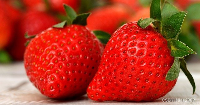
图像2 - 草莓(99.9%)
# Import Pillow
from PIL import Image
img = Image.open("strawberries.jpg")
process_images_by_AlexNet(img)
torch.Size([1, 1000])
strawberry 99.99411010742188
[('strawberry', 99.99411010742188), ('banana', 0.0008383101085200906), ('custard apple', 0.0008333695586770773), ('orange', 0.0007468032999895513), ('lemon', 0.0005674762651324272)]
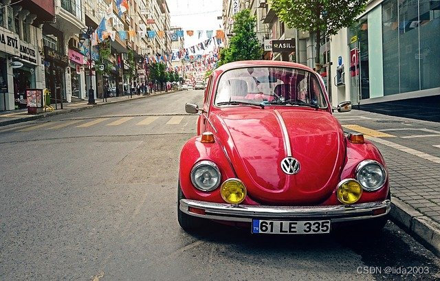
图像3 - 汽车(33.9%)
# Import Pillow
from PIL import Image
img = Image.open("automotive.jpg")
process_images_by_AlexNet(img)
torch.Size([1, 1000])
cab, hack, taxi, taxicab 33.94831466674805
[('cab, hack, taxi, taxicab', 33.94831466674805), ('sports car, sport car', 15.606391906738281), ('racer, race car, racing car', 10.1033296585083), ('beach wagon, station wagon, wagon, estate car, beach waggon, station waggon, waggon', 7.658527851104736), ('convertible', 6.8374223709106445)]
图像4 - 穿越机(识别错误!!!)
尽然识别成了割草机,哈哈!!!估计训练集里面压根没有这个类别,不过确实曾经有“割草”功能!
# Import Pillow
from PIL import Image
img = Image.open("aos5.jpg")
process_images_by_AlexNet(img)
torch.Size([1, 1000])
lawn mower, mower 36.8341064453125
[('lawn mower, mower', 36.8341064453125), ('harvester, reaper', 22.15677833557129), ('half track', 6.54979944229126), ('thresher, thrasher, threshing machine', 4.788162708282471), ('forklift', 3.2068734169006348)]

3.4 ResNet用于图像分类
由于AlexNet和ResNet都是在相同的ImageNet数据集上训练的,我们可以对这两个模型使用相同的方法。 ResNet101是一个拥有 101 层卷积神经网络。ResNet101 在训练过程中调整了约 4450 万个参数。这参数太庞大了!
# First, load the model
resnet = models.resnet101(pretrained=True)

# Second, put the network in eval mode
resnet.eval()
3.4.1 定义图像处理函数
def process_images_by_resnet(img):
    img_t = transform(img)
    batch_t = torch.unsqueeze(img_t, 0)

    # Carry out inference on image1
    out = resnet(batch_t)
    print(out.shape)

    # Load labels
    with open('imagenet_classes.txt') as f:
        classes = [line.strip() for line in f.readlines()]

    _, index = torch.max(out, 1)
    percentage = torch.nn.functional.softmax(out, dim=1)[0] * 100
    print(classes[index[0]], percentage[index[0]].item())

    # Forth, print the top 5 classes predicted by the model
    _, indices = torch.sort(out, descending=True)
    print([(classes[idx], percentage[idx].item()) for idx in indices[0][:5]])
3.4.2 评估推理结果
# We will evaluate dog, strawberries, automotive, and download function is disabled here.
from PIL import Image
img1 = Image.open("dog.jpg")
img2 = Image.open("strawberries.jpg")
img3 = Image.open("automotive.jpg")
img4 = Image.open("aos5.jpg")
图像1 - 拉布拉多犬(48.8%)
process_images_by_resnet(img1)
torch.Size([1, 1000])
Labrador retriever 48.86875915527344
[('Labrador retriever', 48.86875915527344), ('dingo, warrigal, warragal, Canis dingo', 8.17887020111084), ('golden retriever', 6.944704055786133), ('Eskimo dog, husky', 3.563750982284546), ('bull mastiff', 3.0799338817596436)]
图像2 - 草莓(99.7%)
process_images_by_resnet(img2)
torch.Size([1, 1000])
strawberry 99.76702117919922
[('strawberry', 99.76702117919922), ('trifle', 0.02754645235836506), ('pineapple, ananas', 0.013453328981995583), ('strainer', 0.012202989310026169), ('thimble', 0.012185103259980679)]
图像3 - 汽车(86.7%)
process_images_by_resnet(img3)
torch.Size([1, 1000])
sports car, sport car 86.77729797363281
[('sports car, sport car', 86.77729797363281), ('convertible', 8.948866844177246), ('racer, race car, racing car', 1.7048405408859253), ('cab, hack, taxi, taxicab', 1.2756531238555908), ('grille, radiator grille', 0.5685423016548157)]
图像4 - 穿越机(识别错误!!!)
process_images_by_resnet(img4)
torch.Size([1, 1000])
radio, wireless 29.244718551635742
[('radio, wireless', 29.244718551635742), ("carpenter's kit, tool kit", 18.641035079956055), ('power drill', 18.24420738220215), ('joystick', 12.940756797790527), ('mousetrap', 3.2342422008514404)]
4. 分析
到目前为止,已经讨论了如何使用预训练模型进行图像分类,但尚未回答的一个问题是,如何决定为特定任务选择哪个模型。
根据以下标准比较预训练模型:
- Top-1 错误:如果由置信度最高的模型预测的类与真实类不同,则会发生 Top-1 错误。
- Top-5 错误:如果真实类不在模型预测的前 5 个类中(按置信度排序),则会发生 Top-5 错误。
- CPU 推断时间:推断时间是模型推断步骤所需的时间。
- GPU 推断时间:GPU的特殊性,其计算时间应该小于CPU时间
- 模型大小:此处的大小指的是由 PyTorch 提供的预训练模型的 .pth 文件所占据的物理空间。
一个好的模型将具有较低的 Top-1 错误、较低的 Top-5 错误、较低的 CPU 和 GPU 推断时间以及较低的模型大小。
所有实验都在相同的输入图像上进行了多次,以便分析特定模型所有结果的平均值。实验在 Google Colab 上进行。
4.1 模型准确性比较
Top-1错误是指顶级预测类别与真实情况不同。由于问题相当困难,因此还有另一个错误度量称为Top-5错误。如果前5个预测类别都不正确,则将预测分类为错误。
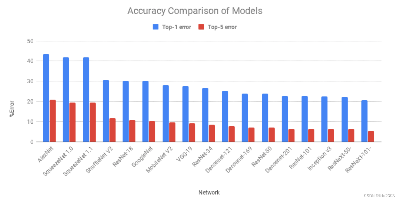 从图表可以看出,这两种错误都呈现出类似的趋势。AlexNet是基于深度学习的第一次尝试,自那时以来,错误率有所改善。
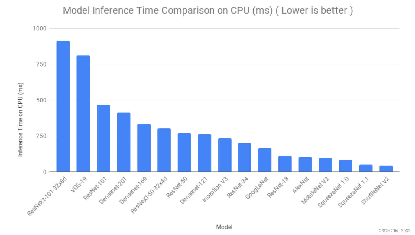
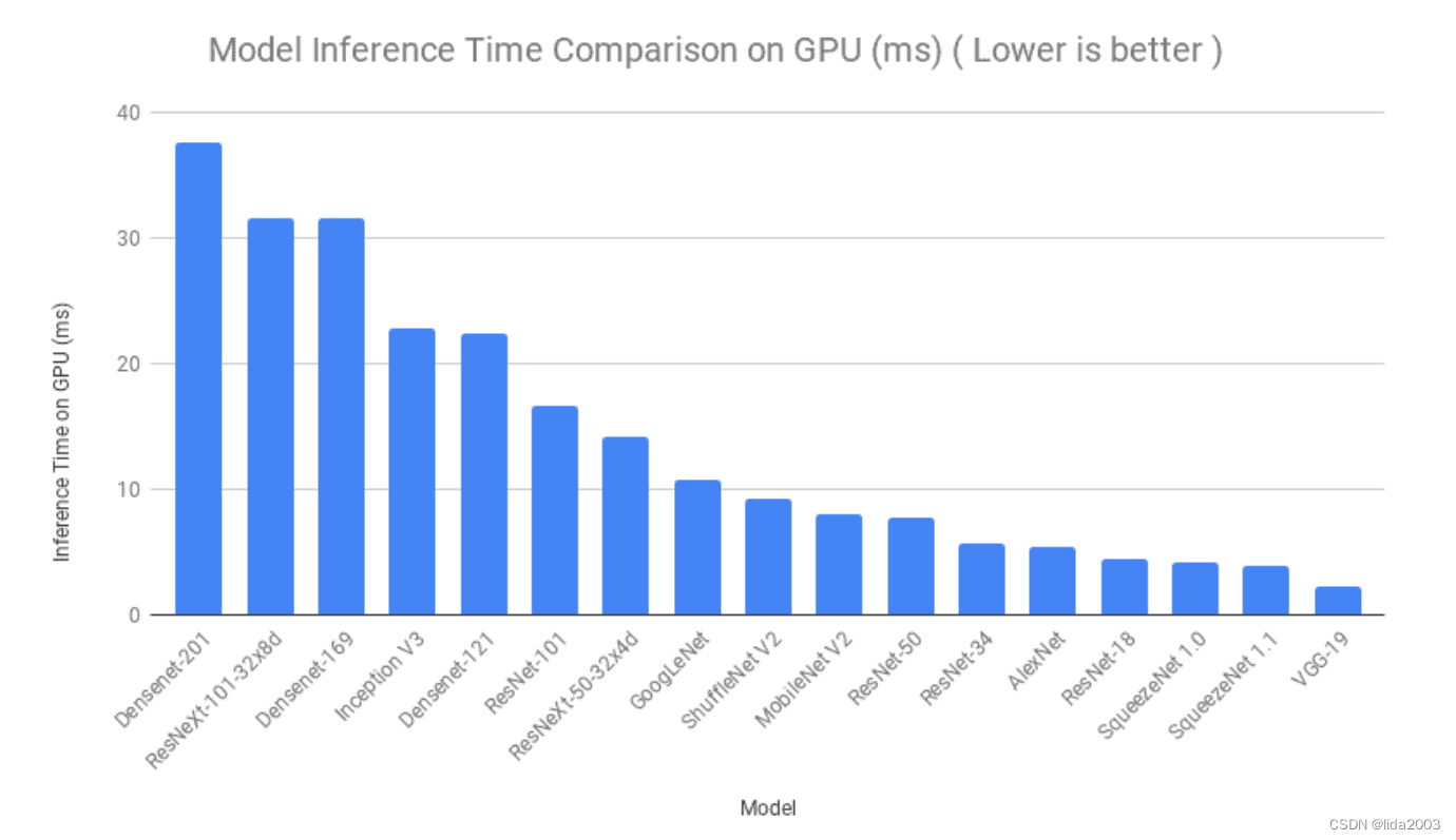
4.2 推断时间比较
接下来,将根据模型推断所需的时间进行比较。每个模型都被提供了相同的图像多次,对所有迭代的推断时间进行了平均。类似的过程在 Google Colab 上针对 CPU 和 GPU 都进行了。尽管在顺序上存在一些变化,但我们可以看到 SqueezeNet、ShuffleNet 和 ResNet-18 的推断时间非常低;GPU都比CPU的耗时低。
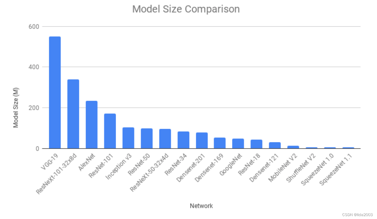
4.3 模型大小比较
很多时候,当我们在安卓或iOS设备上使用深度学习模型时,模型大小成为决定因素,有时甚至比准确性更重要。SqueezeNet 的模型大小最小(5 MB),其次是ShuffleNet V2(6 MB)和MobileNet V2(14 MB)。显而易见的是,这些模型在利用深度学习的移动应用程序中更受青睐的原因。
4.4 总体比较
我们讨论了基于特定标准哪个模型表现更好。我们可以将所有这些重要细节压缩在一个气泡图中,然后根据我们的需求决定选择哪个模型。
我们使用的x坐标是Top-1错误(越低越好)。y坐标是GPU推断时间(毫秒,越低越好)。气泡大小代表模型大小(越低越好)。
- 模型大小较小的气泡更好。
- 靠近原点的气泡在准确性和速度方面都更好。
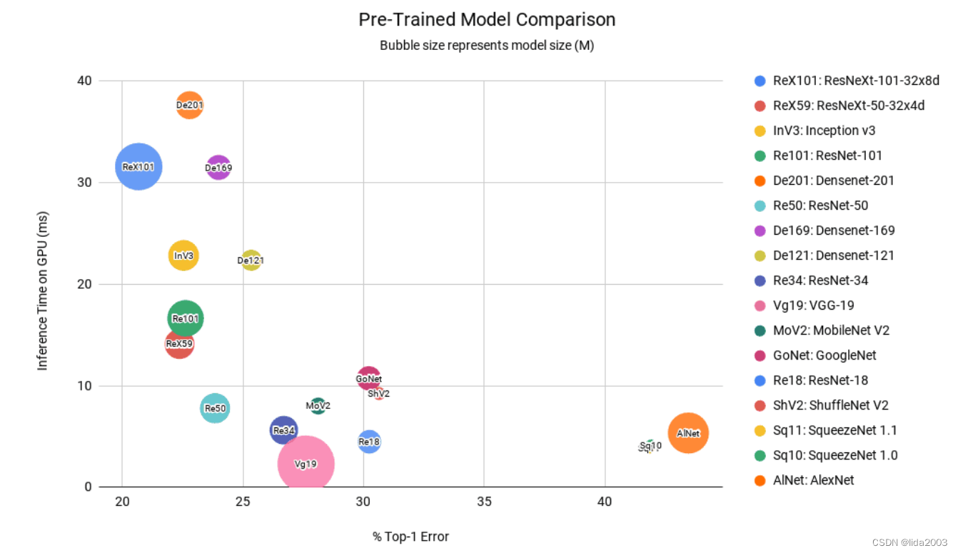
5. 总结
从上图可以清楚地看出,
- ResNet50是在所有三个参数方面(体积小且靠近原点)表现最佳的模型。
- DenseNets 和 ResNext101 在推断时间上较为昂贵。
- AlexNet 和 SqueezeNet 的错误率相当高。
测试代码:002 Pre Trained Models for Image Classification


 被折叠的 条评论
为什么被折叠?
被折叠的 条评论
为什么被折叠?
 到【灌水乐园】发言


